2 Repeated Factors

In the previous class, we saw eating some small amount of chocolate increased the class fixation to the lecture. However, because we took the average fixation over the course the class, we are not sure how the long the effect lasts. To understand how chocolate modulates attention, we designed a 4x3 study fully within-subjects design. During the first 20 min of class, Graduate students’ eyes were tracked. We measured the mean fixation time of student’s eyes on the screen (in seconds per glance). In the next 20 mins, graduate students were given a fun-sized Snickers to encourage them to pay attention. However, we are not sure how to “encourage” students. We could give them more snickers the more time they spend looking at the screen (i.e., Positive reinforcement) or try to encourage them to look back at the screen when they take their eyes off it too long (i.e., Negative reinforcement). The machine continued giving out Snickers for the rest of the class period, depending on the condition they were in during that particular lecture. Finally, we needed a control condition to understand how attention was modulated throughout the 80-minute lecture (No reinforcement). The mean fixation time was recorded and reported at the end of every 20 min interval (for a total of 4 intervals). The order in which students received No, Positive, Negative reinforcement was counterbalanced between the topics of the lecture (“Power Analysis,” “Bootstrapping Theory,” and “Probability Theory,” which were matched based on the thrilling-ness of topic). We will simulated \(n\) = 9 students. If classical learning theory is correct, when students are positively rewarded they will pay more attention to the lecture and when they are negatively rewarded the will learn that they get more chocolate the less they pay attention. However, if graduate students are intrinsically motivated, negative reinforcement might not adversely affect attention as strongly as classical learning theory predicts. Further, we expect fatigue to set in and cause reductions of attention in all conditions.

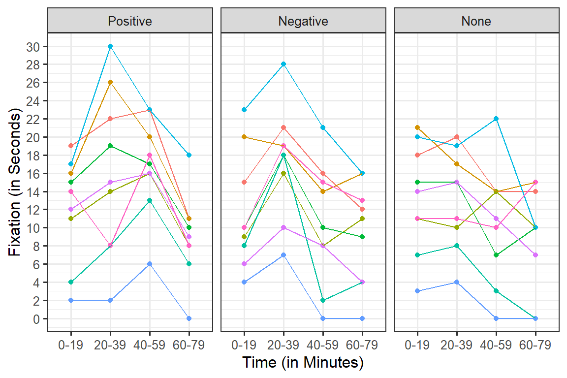
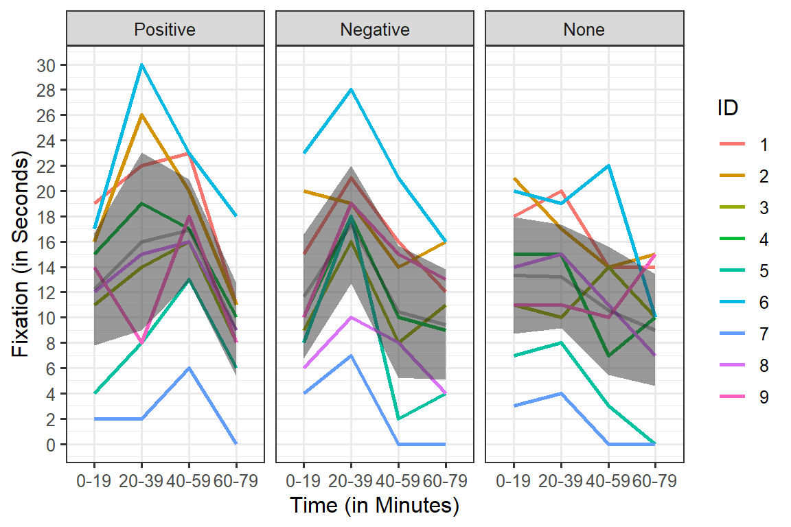
Plot of Simulation

Spaghetti Plot

Each line represents a person’s score across conditions

Means plot

We will plot them as Lines with no error bars for now (plotting error in RM designs is different, and we will come back to that later).

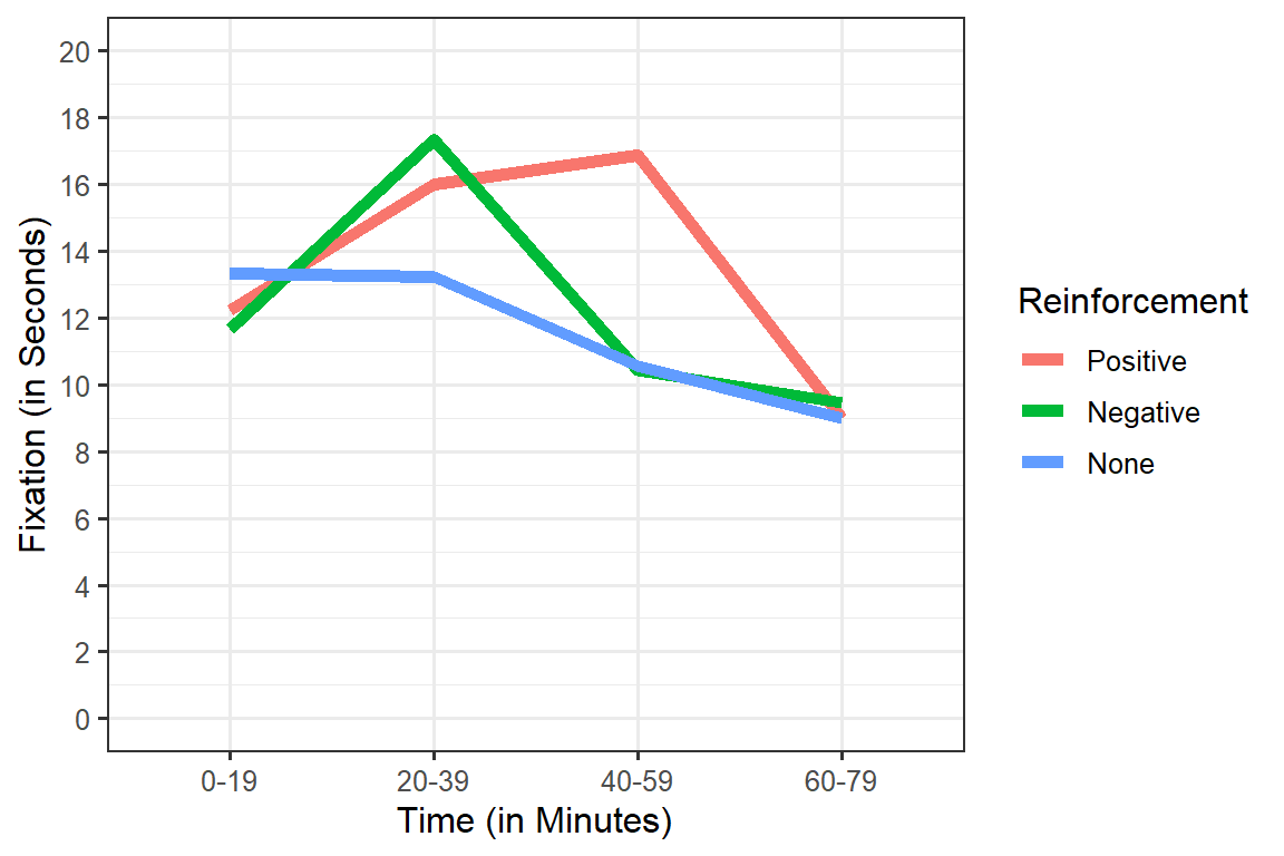
Are there main-effects for Time or Reinforcement and does Time and Reinforcement interact?

2-Way RM ANOVA logic

Just like two-way ANOVA, in the two-way RM ANOVA, you have two Main-effects and an interaction. However, the errors terms are more complicated.
Just as in one-way RM ANOVA we will find the variance due to the individual difference, which we can estimate by calculating the row sum, which are the sums of each subject’s scores.

One-way RM ANOVA Table With the formulas (conceptually simplified)

Source	SS	DF	MS	F
\(RM_1\)	\(nSS_{Treat\,1\,cell\,means}\)	\(C-1\)	\(\frac{SS_{RM}}{df_{RM}}\)	\(\frac{MS_{RM_1}}{MS_{E_1}}\)
Within	\(\displaystyle \sum SS_{within}\)
\(\,Subject\,[Sub]\)	\(\frac{1}{C} SS_{subjects:\, rows\,sums}\)	\(n-1\)	\(\frac{SS_{sub}}{df_{sub}}\)
\(\,Error [Sub\,x\,RM_1]\)	\(SS_W-SS_{sub}\)	\((n-1)(c-1)\)	\(\frac{SS_{E_1}}{df_{E_1}}\)
Total	\(SS_{scores}\)	\(N-1\)

Note: \(SS_{sub} + SS_E = SS_W\) & \(SS_{RM} + SS_W = SS_T\) & \(df_{RM} + df_W = df_T\)

Two-way RM ANOVA Table With the formulas (conceptually simplified)

Source	SS	DF	MS	F
\(RM_1\)	\(C_2nSS_{treat\,1\,cell\,means}\)	\(C_1-1\)	\(\frac{SS_{RM_1}}{df_{RM_1}}\)	\(\frac{MS_{RM_1}}{MS_{E_1}}\)
\(RM_2\)	\(C_1nSS_{treat\,2\,cell\,means}\)	\(C_2-1\)	\(\frac{SS_{RM_2}}{df_{RM_2}}\)	\(\frac{MS_{RM_2}}{MS_{E_2}}\)
\(RM_{1x2}\)	\(nSS_{all\,treat\,cells}-SS_{RM_1} - SS_{RM_2}\)	\((C_1-1)(C_2-1)\)	\(\frac{SS_{RM_{1x2}}}{df_{RM_{1x2}}}\)	\(\frac{MS_{RM_{1x2}}}{MS_{E_{1x2}}}\)
Within	\(\displaystyle \sum SS_{within}\)	\((n-1)(C_1C_2)\)	\(\frac{SS_w}{df_w}\)
\(\,Subject\,[Sub]\)	\(\frac{1}{C_1}\frac{1}{C_2} SS_{subjects:\, rows\,sums}\)	\(n-1\)	\(\frac{SS_{sub}}{df_{sub}}\)
\(\,Error_1 [Sub\,x\,RM_1]\)	\(C_2SS_{treat\,1\,cells}-SS_{RM_1}-SS_{sub}\)	\((n-1)(C_1-1)\)	\(\frac{SS_{E_1}}{df_{E_1}}\)
\(\,Error_2 [Sub\,x\,RM_2]\)	\(C_1SS_{treat\,2\,cells}-SS_{RM_2}-SS_{sub}\)	\((n-1)(C_2-1)\)	\(\frac{SS_{E_2}}{df_{E_2}}\)
\(\,Error_{1x2} [Sub\,x\,RM_{1x2}]\)	\(SS_{w}-SS_{sub}-SS_{E_1}-SS_{E_2}\)	\((n-1)(C_1-1)(C_2-1)\)	\(\frac{SS_{E_{1x2}}}{df_{E_{1x2}}}\)
Total	\(SS_{scores}\)	\(N-1\)

Note:

\(SS_{sub} + SS_{E_1} + SS_{E_2} +SS_{E_{1x2}} = SS_W\)

\(SS_{RM1} + SS_{RM2} +SS_{RM1x2} + SS_W = SS_T\)

\(df_{RM1} + df_{RM2} +df_{RM1x2} + df_W = df_T\)

Explained vs. Unexplained Terms

Explained:

\(SS_{RM_1}\) = caused by treatment 1
\(SS_{RM_2}\) = caused by treatment 2
\(SS_{RM_{1x2}}\) = caused by treatment 1 x treatment 2
\(SS_{sub}\) = individual differences (you do not know why people are different from each other, but you can parse this variance, so we explained it).

Unexplained:

\(SS_{E_1}\) = Noise due to \({RM_1}\)
\(SS_{E_2}\) = Noise due to \({RM_1}\)
\(SS_{E_{1x2}}\) = Noise due to \(RM_{1x2}\)

R ANOVA Calculations

R Defaults

afex calculates the RM ANOVA for us and it will automatically correct for sphericity violations.
Error(Subject ID/RM Factor 1 X RM Factor 2): This tells the afex that subjects vary as function RM conditions.
It reports \(\eta_g^2\) assuming a manipulated treatment.

library(afex)
Model.1<-aov_car(Fixation~ Time*Reinforcement + Error(ID/Time*Reinforcement), 
        data = DataSim2,include_aov = TRUE)
Model.1

## Anova Table (Type 3 tests)
## 
## Response: Fixation
##               Effect          df   MSE         F  ges p.value
## 1               Time 1.91, 15.28 11.59 24.83 *** .129   <.001
## 2      Reinforcement 1.44, 11.49 13.92    3.71 + .020    .068
## 3 Time:Reinforcement 2.94, 23.52 15.16   5.93 ** .066    .004
## ---
## Signif. codes:  0 '***' 0.001 '**' 0.01 '*' 0.05 '+' 0.1 ' ' 1
## 
## Sphericity correction method: GG

Assumptions

Sphericity

Same as one-way ANOVA, except we should examine Mauchly’s test for Sphericity on each term (that has more than 2 levels)

aov_car(Fixation~ Time*Reinforcement + Error(ID/Time*Reinforcement), 
        data = DataSim2, return="univariate")

## 
## Univariate Type III Repeated-Measures ANOVA Assuming Sphericity
## 
##                     Sum Sq num Df Error SS den Df F value    Pr(>F)    
## (Intercept)        16675.6      1  3021.24      8 44.1556 0.0001616 ***
## Time                 549.4      3   177.06     24 24.8259 1.557e-07 ***
## Reinforcement         74.2      2   159.93     16  3.7138 0.0473315 *  
## Time:Reinforcement   264.1      6   356.44     48  5.9264 0.0001093 ***
## ---
## Signif. codes:  0 '***' 0.001 '**' 0.01 '*' 0.05 '.' 0.1 ' ' 1
## 
## 
## Mauchly Tests for Sphericity
## 
##                    Test statistic p-value
## Time                      0.31701 0.17706
## Reinforcement             0.60746 0.17471
## Time:Reinforcement        0.02211 0.41492
## 
## 
## Greenhouse-Geisser and Huynh-Feldt Corrections
##  for Departure from Sphericity
## 
##                     GG eps Pr(>F[GG])    
## Time               0.63670  1.851e-05 ***
## Reinforcement      0.71811   0.068052 .  
## Time:Reinforcement 0.48998   0.003827 ** 
## ---
## Signif. codes:  0 '***' 0.001 '**' 0.01 '*' 0.05 '.' 0.1 ' ' 1
## 
##                       HF eps   Pr(>F[HF])
## Time               0.8314754 1.417163e-06
## Reinforcement      0.8322961 5.871770e-02
## Time:Reinforcement 0.8056227 4.170679e-04

Covariance Matrix

For most RM ANOVAs we assume Compound Symmetry:

\[ \mathbf{Cov} = \sigma^2\left[\begin{array} {rrrr} 1 & \rho & \rho & \rho \\ \rho & 1 & \rho & \rho \\ \rho & \rho & 1 & \rho \\ \rho & \rho & \rho & 1\\ \end{array}\right] \]

However, as in the case of the study that we examined today, people do not always behave over time the with the same correction over time. This about a longitudinal study where time can be over weeks or months. Time introduces a strange problem called ‘auto-regression’ (auto-correlation), i.e., what I do now impacts what I do next (remember Time cannot be counterbalanced).

There are many other types of Covariance Matrices that you can assume, but not in RM ANOVA. RM ANOVA is a special case of the linear mixed model. Next semester will explore linear mixed models a little, which are better for dealing with time.

Here is an example of Covariance Matrix specifically meant for time: First Order Autoregressive AR(1):

\[ \mathbf{Cov} = \sigma^2\left[\begin{array} {rrrr} 1 & \rho & \rho^2 & \rho^3 \\ \rho & 1 & \rho & \rho^2 \\ \rho^2 & \rho & 1 & \rho \\ \rho^3 & \rho^2 & \rho & 1\\ \end{array}\right] \]

Plot Results

Problems with Error Bars

Within-subject designs present a few problems when plotting “error” for a visual approximation of significance. The main problem is that we are plotting the error within each cell (the individual differences). The gray band over the data is the 95%CI.

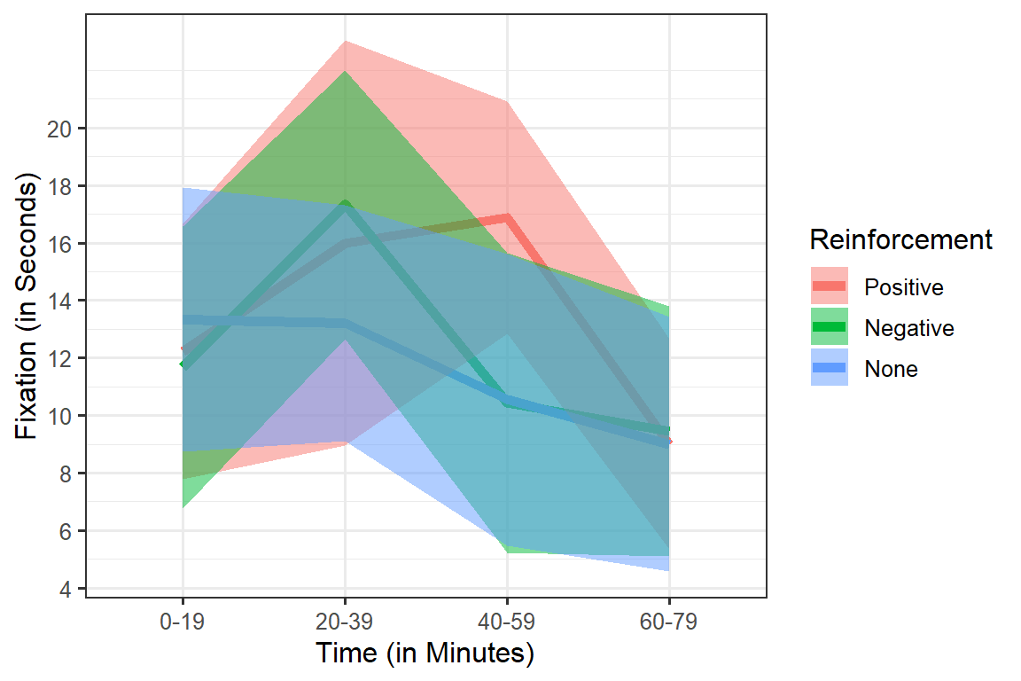
Non-Corrected Error Bars

When we collapse the lines and plot the CIs, we can see they completely overlap. We might conclude there are no significant differences between the groups. But again the problem is we have not removed the individual differences (which we can account for).

Within Errors Bars: CI

We will use Cousineau-Morey Corrected error bars which remove individual differences (see Morey, 2008 Figure 1 for visual of the difference between error bar types & Cousineau & O’Brien, 2014 for a review on the theory). First, we center each subject (remove their means across all conditions). This makes each person’s mean = 0 (across conditions). Next, we recalculate the standard error or confidence interval on these centered means. Finally, we apply a correction to correct for bias (this method underestimates the variance). Correction = \(\sqrt{\frac{J}{J-1}}\), where J = number of within factors. Correct SE for plotting = SE (or CI) on centered data * Correction.

This is a lot of steps, so Cousineau & O’Brien (2014) provide some sample code. Also, there is a function built into the afex package that will produce this correction (see https://www.rdocumentation.org/packages/afex/versions/0.22-1/topics/afex_plot). However, I find it easier to use the function supplied by http://www.cookbook-r.com/Graphs/Plotting_means_and_error_bars_(ggplot2)/.

Note: I have adapted their code so that it does not conflict with dplyr code. So use the corrected functions I have supplied you otherwise if you are trying to use dplyr it will break (as this function requires the older plyr package. You will need to install plyr package, but do NOT load it). You have to be very careful when using the plyr and dplyr package at the same time.

To use this function, you have to load the scripts (set the working directory where the file lives and source the file)

You can plot corrected +/- 1 SE or 95%CIs. Below is 95%CI. Compare them to the uncorrected 95% CI above. The difference here is not massive,

#setwd("C:/Users/ademos/Dropbox/AlexFiles/teaching/UIC/Graduate/543-Fall2021/Week 9")

source('HelperFunctions.R')

MeansforGGPlot <- summarySEwithin(data=DataSim2, "Fixation", withinvars=c("Time","Reinforcement"),
                            idvar="ID", na.rm=FALSE, conf.interval=.95)

Means.Within.CI <-ggplot(data = MeansforGGPlot, aes(x = Time, y=Fixation, group=Reinforcement))+
  scale_y_continuous(breaks = seq(0,20,2))+
  geom_line(aes(colour = Reinforcement), size=2)+
  geom_ribbon(aes(ymin=Fixation-ci, ymax=Fixation+ci,fill = Reinforcement), alpha=.5)+
  ylab("Fixation (in Seconds)")+xlab("Time (in Minutes)")+
  theme(legend.position = "right")
Means.Within.CI

For within error bars (Corrected) you can eye-ball significance (Cumming & Finch, 2005)

95% CIs:

\(p < .05\): when proportion overlap is about .50
\(p < .01\): when proportion overlap is about 0

Within Errors Bars: SE

Means.Within.SE <-ggplot(data = MeansforGGPlot, aes(x = Time, y=Fixation, group=Reinforcement))+
  scale_y_continuous(breaks = seq(0,20,2))+
  geom_line(aes(colour = Reinforcement), size=2)+
  geom_ribbon(aes(ymin=Fixation-se, ymax=Fixation+se,fill = Reinforcement), alpha=.5)+
  ylab("Fixation (in Seconds)")+xlab("Time (in Minutes)")+
  theme(legend.position = "right")
Means.Within.SE

SE bars:

\(p < .05\): when proportion gap is 1x size of SE bar
\(p < .01\): when proportion gap is 2x size of SE bar

Follow Up Testing

Following up the main-effects and interactions are mostly the same as with two-way ANOVA. However, you have a few more decision to make based on how conservative you want to be.

What are your assumption?

Do you assume strong violations sphericity? You can approach it two different ways.
- 1. Only do pairwise t-tests (ignore omnibus RM ANOVA)
- 1. Use the a MANOVA (Multivariate ANOVA) for error variance and do contrasts as usual (default approach in AFEX as of version 1.0, to match SPSS)
Do you assume no or small violations sphericity?

Assume Strong Violations of Sphericity: Univariate Classical Approach

Your book recommends simply not using the errors term from the ANOVAs and running pairwise comparisons ONLY using paired t-tests, Bonferroni corrected. This is the oldest and still common approach. The problem with this approach, you cannot do anything but pairwise analysis (no contrasts of any kind).

Pros:

Protects Type I error the best

Cons:

MASSIVE inflation of Type II error
You cannot do any type of contrast you want (you can only do pairwise or stepwise)

Follow-up Interaction

Its best to examine things within simple effects (so lets look at time pairwise within each level of Time). This is a total of 12 tests and will tell me at each timepoint when the reinforcements seperate.

Using the pairwise.t.test, we pass it the arguments paired=TRUE and p.adj = "bonf" (Note: this is one family of tests, so \(a_{bon} = .05 / 12 = 0.0042\)

library(broom)
library(dplyr)
DataSim2 %>% 
  group_by(Time) %>% 
  do(
    tidy(
    pairwise.t.test(.$Fixation,.$Reinforcement,
                    paired=TRUE,
                    p.adj = "bonf")))

## # A tibble: 12 × 4
## # Groups:   Time [4]
##    Time  group1   group2    p.value
##    <fct> <chr>    <chr>       <dbl>
##  1 0-19  Negative Positive 1       
##  2 0-19  None     Positive 0.618   
##  3 0-19  None     Negative 0.523   
##  4 20-39 Negative Positive 1       
##  5 20-39 None     Positive 0.355   
##  6 20-39 None     Negative 0.0915  
##  7 40-59 Negative Positive 0.000287
##  8 40-59 None     Positive 0.00122 
##  9 40-59 None     Negative 1       
## 10 60-79 Negative Positive 1       
## 11 60-79 None     Positive 1       
## 12 60-79 None     Negative 1

Effect sizes

Just run Cohen’s d (again ignore error term of ANOVA). Code broken working on it…

Assume Strong Violations of Sphericity: Multivariate Approach

You can choose instead to do what SPSS does by default for contrasts: assume violations of sphericity. This uses a different approach (multivariate analysis) and uses smaller more conservative DF (we will not get to deep into the details of univariate vs. multivariate testing yet). This is a conservative approach.

Pros:

You can apply an extra correction (HSD, MVT, Sidek, Holm, Bonferroni, etc.)
You can do any type of contrast you want
Protects Type I error better

Cons:

Can inflate Type II

Error term and DF do NOT come from the RM ANOVA. The come from a MANOVA (Multivariate analysis of variance) instead. This assumes your repeated measures are actually multiple (but independent) measures from the same subject (like three different ways of asking about a similar construct). MANOVA “eats” all your DF (now we use \(df_E = n-1\)) and its less powerful overall (so more type II errors) as the MANOVA does not assume Sphericity (but does account for the covariance between measures). If we run a MANOVA on the data we will get Pillai test (0-1; which term is contributing more to the overall model), but also it will give us an “approximate F”.

MANOVA results vs ANOVA

library(afex)
Model.1<-aov_car(Fixation~ Time*Reinforcement + Error(ID/Time*Reinforcement), 
        data = DataSim2,include_aov = TRUE)
Model.1

Model.M<-aov_car(Fixation~ Time*Reinforcement + Error(ID/Time*Reinforcement), 
        data = DataSim2, return='Anova')
Model.M

## Anova Table (Type 3 tests)
## 
## Response: Fixation
##               Effect          df   MSE         F  ges p.value
## 1               Time 1.91, 15.28 11.59 24.83 *** .129   <.001
## 2      Reinforcement 1.44, 11.49 13.92    3.71 + .020    .068
## 3 Time:Reinforcement 2.94, 23.52 15.16   5.93 ** .066    .004
## ---
## Signif. codes:  0 '***' 0.001 '**' 0.01 '*' 0.05 '+' 0.1 ' ' 1
## 
## Sphericity correction method: GG 
## 
## Type III Repeated Measures MANOVA Tests: Pillai test statistic
##                    Df test stat approx F num Df den Df    Pr(>F)    
## (Intercept)         1   0.84661   44.156      1      8 0.0001616 ***
## Time                1   0.84417   10.835      3      6 0.0077775 ** 
## Reinforcement       1   0.71212    8.658      2      7 0.0128015 *  
## Time:Reinforcement  1   0.92804    6.448      6      3 0.0773454 .  
## ---
## Signif. codes:  0 '***' 0.001 '**' 0.01 '*' 0.05 '.' 0.1 ' ' 1

What you can see the interaction is no longer significant at \(p <.05\), so we would not follow it up. However, people often do NOT look at the MANOVA results. They look at the RM ANOVA results and follow that up assuming MANOVA. Its totally logically inconsistent, but that is what SPSS users do and thats what most people are use too.

You don’t need to actually run or look at the MANOVA results. You will pass emmeans the orginal Afex object (as its has the MANOVA in it already).

Follow Up Interaction

Example using simple effects followed up by pairwise comparisons

library(emmeans)
Reinforcement.by.Time.M<-emmeans(Model.1,~Reinforcement|Time, model = "multivariate")
joint_tests(Reinforcement.by.Time.M, by = "Time")

## Time = X0.19:
##  model term    df1 df2 F.ratio p.value
##  Reinforcement   2   8   2.658  0.1303
## 
## Time = X20.39:
##  model term    df1 df2 F.ratio p.value
##  Reinforcement   2   8   4.469  0.0498
## 
## Time = X40.59:
##  model term    df1 df2 F.ratio p.value
##  Reinforcement   2   8  30.403  0.0002
## 
## Time = X60.79:
##  model term    df1 df2 F.ratio p.value
##  Reinforcement   2   8   0.203  0.8205

Since we see only the middle two-time points had differences, we will examine the pairwise results within each family (note you can do any custom contrast you want). You also need to decide what correlation you want to apply.

pairs(Reinforcement.by.Time.M, adjust ='tukey')

## Time = X0.19:
##  contrast            estimate    SE df t.ratio p.value
##  Positive - Negative    0.556 1.519  8   0.366  0.9296
##  Positive - None       -1.111 0.807  8  -1.377  0.3964
##  Negative - None       -1.667 1.118  8  -1.491  0.3448
## 
## Time = X20.39:
##  contrast            estimate    SE df t.ratio p.value
##  Positive - Negative   -1.333 2.088  8  -0.638  0.8038
##  Positive - None        2.778 1.588  8   1.749  0.2463
##  Negative - None        4.111 1.567  8   2.623  0.0706
## 
## Time = X40.59:
##  contrast            estimate    SE df t.ratio p.value
##  Positive - Negative    6.444 0.899  8   7.167  0.0002
##  Positive - None        6.333 1.093  8   5.795  0.0010
##  Negative - None       -0.111 1.086  8  -0.102  0.9942
## 
## Time = X60.79:
##  contrast            estimate    SE df t.ratio p.value
##  Positive - Negative   -0.444 1.132  8  -0.393  0.9193
##  Positive - None        0.000 1.590  8   0.000  1.0000
##  Negative - None        0.444 0.988  8   0.450  0.8958
## 
## P value adjustment: tukey method for comparing a family of 3 estimates

Assume no or small Violations of Sphericity: Univariate Approach

emmeans sort of uses the error terms from the ANOVA (but actually calculated the pooled variance of the difference scores per comparisons). For the interaction calculates degrees of freedom based on Satterthwaite approximations (somewhat correct for HOV). However, this does not control for violations of sphericity. So when you have violations of sphericity, this approach is anti-conservative and can inflate type I error on follow-ups. When sphericity is not violated, this approach is equivalent protected t-tests.

Pros:

You can apply an extra correction (HSD, MVT, Sidek, Holm, Bonferroni, etc.)
You can do any type of contrast you want

Cons:

Can inflate type I error (worse so when sphericity is violated)

Follow Up Interaction

Example using simple effects followed up by pairwise comparisons

library(emmeans)
Reinforcement.by.Time.UV<-emmeans(Model.1,~Reinforcement|Time,model = "univariate" )
joint_tests(Reinforcement.by.Time.UV, by = "Time")

## Time = X0.19:
##  model term    df1   df2 F.ratio p.value
##  Reinforcement   2 62.81   0.803  0.4524
## 
## Time = X20.39:
##  model term    df1   df2 F.ratio p.value
##  Reinforcement   2 62.81   4.907  0.0105
## 
## Time = X40.59:
##  model term    df1   df2 F.ratio p.value
##  Reinforcement   2 62.81  15.181  <.0001
## 
## Time = X60.79:
##  model term    df1   df2 F.ratio p.value
##  Reinforcement   2 62.81   0.073  0.9293

Since we see only the middle two-time points had differences.

Pairs.UV<-pairs(Reinforcement.by.Time.UV, adjust ='tukey')
Pairs.UV

## Time = X0.19:
##  contrast            estimate   SE   df t.ratio p.value
##  Positive - Negative    0.556 1.34 62.8   0.415  0.9096
##  Positive - None       -1.111 1.34 62.8  -0.830  0.6861
##  Negative - None       -1.667 1.34 62.8  -1.245  0.4317
## 
## Time = X20.39:
##  contrast            estimate   SE   df t.ratio p.value
##  Positive - Negative   -1.333 1.34 62.8  -0.996  0.5823
##  Positive - None        2.778 1.34 62.8   2.074  0.1034
##  Negative - None        4.111 1.34 62.8   3.070  0.0087
## 
## Time = X40.59:
##  contrast            estimate   SE   df t.ratio p.value
##  Positive - Negative    6.444 1.34 62.8   4.813  <.0001
##  Positive - None        6.333 1.34 62.8   4.730  <.0001
##  Negative - None       -0.111 1.34 62.8  -0.083  0.9962
## 
## Time = X60.79:
##  contrast            estimate   SE   df t.ratio p.value
##  Positive - Negative   -0.444 1.34 62.8  -0.332  0.9411
##  Positive - None        0.000 1.34 62.8   0.000  1.0000
##  Negative - None        0.444 1.34 62.8   0.332  0.9411
## 
## P value adjustment: tukey method for comparing a family of 3 estimates

Effect sizes

You need to very carefully select the correct error term. If you follow up the interaction, take the interaction error term (the edf to match what ever DF the contrast reads out. This is not correct, but I am not sure yet what to enter)

SD.I = sqrt(Model.1$anova_table$MSE[3])
eff_size(Pairs.UV, sigma = SD.I, edf =62.8, method='identity') %>% summary()

## Time = X0.19:
##  contrast              effect.size    SE   df lower.CL upper.CL
##  (Positive - Negative)      0.1427 0.344 62.8  -0.5451    0.831
##  (Positive - None)         -0.2854 0.345 62.8  -0.9747    0.404
##  (Negative - None)         -0.4281 0.346 62.8  -1.1197    0.263
## 
## Time = X20.39:
##  contrast              effect.size    SE   df lower.CL upper.CL
##  (Positive - Negative)     -0.3425 0.345 62.8  -1.0326    0.348
##  (Positive - None)          0.7135 0.350 62.8   0.0145    1.413
##  (Negative - None)          1.0560 0.357 62.8   0.3433    1.769
## 
## Time = X40.59:
##  contrast              effect.size    SE   df lower.CL upper.CL
##  (Positive - Negative)      1.6554 0.374 62.8   0.9073    2.403
##  (Positive - None)          1.6269 0.373 62.8   0.8808    2.373
##  (Negative - None)         -0.0285 0.344 62.8  -0.7159    0.659
## 
## Time = X60.79:
##  contrast              effect.size    SE   df lower.CL upper.CL
##  (Positive - Negative)     -0.1142 0.344 62.8  -0.8018    0.574
##  (Positive - None)          0.0000 0.344 62.8  -0.6874    0.687
##  (Negative - None)          0.1142 0.344 62.8  -0.5735    0.802
## 
## sigma used for effect sizes: 3.893 
## Confidence level used: 0.95

Follow Up Main-effect

Trend analysis of Time. Note you have to do this BY HAND for the effect sizes to make sense.

Time.Main.Effect<-emmeans(Model.1,~Time,model = "univariate" )
Time.Main.Effect
Poly.Time<-contrast(Time.Main.Effect, 'poly')

##  Time   emmean   SE   df lower.CL upper.CL
##  X0.19   12.41 1.92 8.95     8.05     16.8
##  X20.39  15.52 1.92 8.95    11.16     19.9
##  X40.59  12.63 1.92 8.95     8.27     17.0
##  X60.79   9.15 1.92 8.95     4.79     13.5
## 
## Results are averaged over the levels of: Reinforcement 
## Warning: EMMs are biased unless design is perfectly balanced 
## Confidence level used: 0.95

Effect sizes for Poly = Still working on the code.

Guidelines

Graph your results with the corrected error bars and try to look at spaghetti plots as well. This is MOST important thing you can do in a repeated measure design. You will see the violations of your assumptions, and this will guide your selection of an approach for follow-up testing. You will see bad subjects, conditions, or interactions between subjects and conditions. This way when understanding how your ANOVA will parse your variance.
Design RM studies with tend analyses in mind (think ordinally when possible). When this is not possible make sure to limit the number of levels you will examine. Each level you add the more chance to violate sphericity and inflate Type I error.

Follow-Ups:

When you use the more powerful univariate approach when possible, you must report which packages you use in your method section.
Apply alpha correction and use a more conservative approach over the between-subjects test.
If you use the Old-school method: Avoid using the error term from the RM ANOVA for pairwise testing.
- Yes, it buys power, but at a large cost of Type I error.
  - Do as few tests as you can and thus Bonferroni corrections are not killing you power.

References

Bakeman, R. (2005). Recommended effect size statistics for repeated measures designs. Behavior research methods, 37(3), 379-384.

Cousineau, D., & O’Brien, F. (2014). Error bars in within-subject designs: a comment on Baguley (2012). Behavior Research Methods, 46(4), 1149-1151.

Olejnik, S., & Algina, J. (2003). Generalized eta and omega squared statistics: Measures of effect size for some common research designs. Psychological Methods, 8(4), 434-447. doi:10.1037/1082-989X.8.4.434

RM ANOVA - Two-way, Graphing & Follow ups

2 Repeated Factors

Plot of Simulation

Spaghetti Plot

Means plot

2-Way RM ANOVA logic

One-way RM ANOVA Table With the formulas (conceptually simplified)

Two-way RM ANOVA Table With the formulas (conceptually simplified)

Explained vs. Unexplained Terms

R ANOVA Calculations

R Defaults

Assumptions

Sphericity

Covariance Matrix

Plot Results

Problems with Error Bars

Non-Corrected Error Bars

Within Errors Bars: CI

Within Errors Bars: SE

Follow Up Testing

What are your assumption?

Assume Strong Violations of Sphericity: Univariate Classical Approach

Follow-up Interaction

Effect sizes

Assume Strong Violations of Sphericity: Multivariate Approach

MANOVA results vs ANOVA

Follow Up Interaction

Assume no or small Violations of Sphericity: Univariate Approach

Follow Up Interaction

Effect sizes

Follow Up Main-effect

Guidelines

Follow-Ups:

References