Follow Up to One-way ANOVAs

Experimentwise Error Rate

Experimentwise Error Rate is the likelihood that you will make at least 1 type I error in your experiment (per comparison (\(\alpha_{pc}\))) as you run more and more t-tests.

\[ \alpha_{EW} = 1-(1-\alpha_{pc})^j\]

where, j = # of comparisons

\[ j = \frac{K(K-1)}{2} \]

[Assuming conditional probability, each comparison is independent, and sampling with replacement]

We call this Experimentwise Error Rate (\(\alpha_{EW}\)). If we set \(\alpha_{pc}\) = .05 and \(K\) = increasing from 2 to 15 we can see what happens when we have K number of conditions and we want to make all pairwise comparisons (all cells to all cells)

Aew <-function(alpha,K){1-(1-alpha)^(K*(K-1)/2)} 
K=seq(2,15)
Aew.Report<-mapply(Aew, alpha=.05, K)

plot(K,Aew.Report, type='l', 
     xlab = "# of Conditions", ylab="Experimentwise Error Rate", ylim=c(0,1))
abline(h=.05, col='red')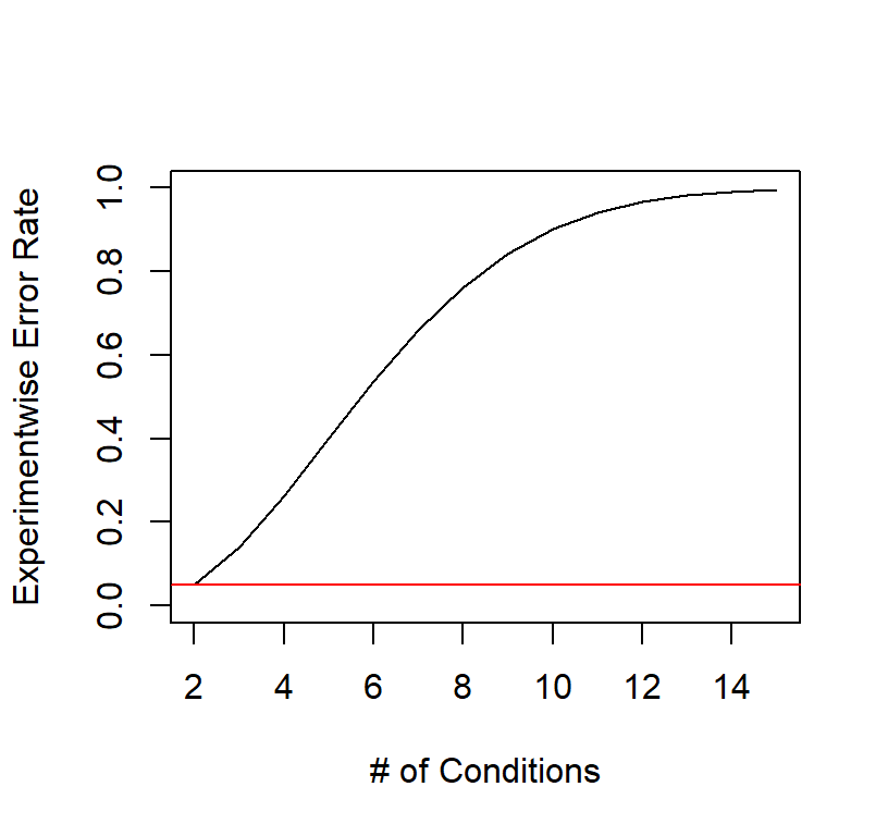

You can see as we do and more tests, we are very likely to commit a type I error.

Familywise error

This is similar to Experimentwise error, but the idea is how much type I error you will get within a “family” of tests. A family of tests will make more sense when we get to two-way ANOVA follow-ups, but in my example at the end I decided that my planned contrasts were one family of tests and my unplanned contrasts were a different family of tests. The logic will become more apparent later this semester.

[Note: Experimentwise is also called Familywise error]

Design Example 1 for Last Class

Interested in how ‘trusting’ of their partner people feel after engaging in various levels of joint action. 2 People enter the lab (one is a confederate) and are asked to either a) move chairs independently, b) Move a couch together, and confederate helps c) Move a couch together and confederate hinders. Moving a couch requires the two people to coordinate their actions. After the study ends, people rate how trustworthy their partner seems (1-7, with 7 = high trust).

No Joint Action	Helpful Joint Action	Disrupted Joint Action
2	5	2
3	4	3
5	7	3
3	4	1
2	5	1
M = 3	M = 5	M = 2

Run ANOVA

library(afex) # 

ANOVA.Table<-aov_car(DV~Condition + Error(SubNum), 
                  data=JA.Study)
ANOVA.Table

## Anova Table (Type 3 tests)
## 
## Response: DV
##      Effect    df  MSE       F  ges p.value
## 1 Condition 2, 12 1.33 8.75 ** .593    .005
## ---
## Signif. codes:  0 '***' 0.001 '**' 0.01 '*' 0.05 '+' 0.1 ' ' 1

So, we need to track down which groups are different.

Which groups are different?

If we run 3 t-tests at an \(\alpha_{pc}\) = .05, we risk (J=3), \(\alpha_{EW}\) = 0.143.

Philosophy I (Familywise) Correction for Error Rate

Dominant Philosophy in Experimental Psychology (Not Neuroscience; We do that next week)

Declared	Null is True (no difference)	Null is False (difference)	Total
Sig	Type 1 (V)	True Positives (S)	R
Non-Sig	True Negative (U)	Type II (T)	m-R
Total	Mo	M-Mo

V / Mo = Probability of getting at least one wrong: we want to keep this at 5%

Different correction methods proposed over the years: From the most anti-conservative to most conservative. They come in and out of favor based on the fashion of the times within each subfield.

Approaches to Follow up

Confirmatory: Hypothesis Driven follow-up

Preferred approach: Look at only those conditions that you predicted would be different. That means you must carefully formulate your predictions. This is hard and will take a long time to learn. It causes people the most frustration. It is required for pre-registered reports and is being required more and more by reviewers. We are starting to leave the dark ages where reviewers would ask for everything to be compared to everything (because type I error problems are being better understood).

• Pros: You will do fewer tests and commit less type 1 errors. Since you run fewer tests, your follow-ups could be more anti-conservative so less type II errors as well (as you will see below).
  
• Cons: You might miss something interesting (but a lot of people argue that those interesting things you find are what ended up causing the replication crisis)

Summary: Low Type I & Low Type II, but risk missing something novel (assuming it’s not type I)

Exploratory: Test everything approach

Out of Favor: Tests all comparisons and/or anything you find interesting. This is the easiest to understand and was a common approach, but is getting hard to publish. Requires very conservative follow up approaches because the risk of Type I is very high.

• Pros: You see everything
• Cons: If you don’t do it correctly most of what you find will be Type I. If you do it correctly, you will commit lots of Type II errors.

Summary: If you do it correctly, Low Type I and super high Type II. If you do it incorrectly, super high Type I and low Type II.

Hybrid approach

Happy Medium?: Do the Confirmatory approach (planned comparisons). Test anything exploratory as conservatively as you can (unplanned comparisons). You need to carefully distinguish what you are doing to your reader otherwise, they will be confused if they are not too statistically savvy as it will seem you are choosing different corrections for unknown reasons.

Contrasts

Contrast as a way of customizing what you want to compare. It is the best way to do Confirmatory testing. You can do pairwise comparisons or more complex testing (merging groups and comparing). This is a huge topic and we will cover only the basic types today and return to advanced forms later in the semester (such as orthogonal and polynomial testing).

Linear Contrast

This is basically an F-test, where you compare only the groups you want to compare on the fly [also allows you do merge groups on the fly].

\[F_{contrast} = \frac{MS_{contrast}}{MS_W} \] Note: your book says:

\[F_{contrast} = \frac{SS_{contrast}}{MS_W} \]

That is correct because \(df_{contrast}\) will always equal 1, because we can only compare 2 groups at once (\(2-1 = 1\)). Thus \(MS_{contrast} = \frac{SS_{contrast}}{1}\). Mathematically, we can skip the \(MS_{contrast}\) step because \(MS_{contrast} = SS_{contrast}\)

Pairwise (linear) Contrast

Step 1

Decide on how you want to weight (we call it \(C\)) your cells (they must add up to zero). I want to compare No vs Helpful (H1) and No vs Disrupted (H2) + Helpful vs Disrupted (H3). The numbers you pick are arbitrary.

If we do three H tests, this is called a family. So we can review the code above to see what our error would be for three tests (\(\alpha_{EW}\) = 0.143)

Cell	No Joint Action	Helpful Joint Action	Disrupted Joint Action	Sum
\(M\)	3	5	2
\(C_{H1}\)	-1	1	0	0
\(C_{H2}\)	-1	0	1	0
\(C_{H3}\)	0	-1	1	0

Step 2

Linear Sum (\(L_{H1}\))

\[ L = \displaystyle\sum_{i=1}^{k}C_iM_i\] \[ L = -1*3 + 1*5 + 0*2 = 2 \]

Step 3

Calculate the \(MS\)/\(SS_{contrast}\)

\[MS_{contrast} = \frac{nL^2}{\sum{C^2}}\]

\[MS_{contrast} = \frac{nL^2}{\sum{C^2}} = \frac{5*2^2}{{(-1)^2+(1)^2+(0)^2}} = \frac{20}{2} = 10\]

Step 4

Calculate \(F_{contrast}\)

\[F_{contrast} = \frac{MS_{contrast}}{MS_W} = \frac{10}{1.33} = 7.5\]

Note: You can convert it to \(t\) like this

\[\sqrt{F_{contrast}} = t_{contrast}\]

\[\sqrt{7.5} = 2.739\]

Step 5

Look up \(F_{crit}\) using this df formula = \((1,df_w)\) or \(t_{crit}\) using this df formula = \((df_w)\)

Doing Contrasts in R

The error term from the ANOVA will be brought into the contrast using the emmeans package (Estimated Marginal Means: When we get to two way ANOVAs you will understand what we mean by Marginal Means alittle better). We need first to run our ANOVA and bring down the ANOVA object from afex. Estimated marginal means are based on a model (thus we will examine the model’s estimates of the fitted values; not the raw data). [ANOVA is a special case of regression, so this method works for regression analysis as well]

library(emmeans)
Fitted.Model<-emmeans(ANOVA.Table, ~Condition)
Fitted.Model

##  Condition  emmean    SE df lower.CL upper.CL
##  Distrupted      2 0.516 12    0.875     3.13
##  Helpful         5 0.516 12    3.875     6.13
##  No              3 0.516 12    1.875     4.13
## 
## Confidence level used: 0.95

You will notice we created a new object that have emmeans (means per cell), the SE (which is the same for all cells because its created from \(MS_W\), when sample sizes are equal \(SE = \frac{MS_w}{\sqrt{n}}\)), \(df_w\) term, and CIs.

We need to pay attention to the order of the object. It does not match our table (so be careful).

Set up the hypotheses (make sure the order matches your fitted emmeans object!)

set1 <- list(
  H1_No.VS.H = c(0,1,-1),
  H2_No.VS.D = c(1,0,-1),
  H3_D.VS.H = c(-1,1,0))

Check: Do they each sum to zero?

c(sum(set1$H1_No.VS.H),sum(set1$H2_No.VS.D),sum(set1$H3_D.VS.H))

## [1] 0 0 0

Run the contrast (adjust = “none”, means don’t correct the pvalue for multiple comparisons).

contrast(Fitted.Model, set1, adjust = "none") %>% summary(infer = TRUE)

##  contrast   estimate   SE df lower.CL upper.CL t.ratio p.value
##  H1_No.VS.H        2 0.73 12    0.409    3.591   2.739  0.0180
##  H2_No.VS.D       -1 0.73 12   -2.591    0.591  -1.369  0.1960
##  H3_D.VS.H         3 0.73 12    1.409    4.591   4.108  0.0015
## 
## Confidence level used: 0.95

It matches the by-hand calculation!

Pairwise contrast = Fisher’s Protected t-test (aka LSD)

LSD = Least Significant Difference is the most anti-conservative as it provides almost no protection on type I error (but its used as the base pairwise method for other approaches). It corrects the t-test formula directly:

\[ t = \frac{M_1 - M_2} {\sqrt{\frac{S^2_p}{n_1}+ \frac{S^2_p}{n_2}}}\]

\[LSD= \frac{M_1 - M_2} {\sqrt{\frac{MS_W}{n_1}+ \frac{MS_W}{n_2}}} \]

This works because \(MS_W\) is basically \(S^2_p\), in that \(MS_W\) is the pooled variance term (but across all groups), where \(S^2_p\) is just between the groups of interest. This is because the error term contains the pooled variance of all group, so its safer version of the t-test formula for our follow up tests.

LSD is only appropriate when you are doing Confirmatory testing with 3 or less comparisons

\[LSD_{SE}= \sqrt{\frac{MS_W}{n_1}+ \frac{MS_W}{n_2}}\]

\[LSD_{SE}= \sqrt{\frac{1.33}{5}+ \frac{1.33}{5}}\]

\(LSD_{SE}= .73\), which matched our contrast SE.

Doing LSD in R

LSD can be done automatically and is little easier than writing the linear contrast.

Fitted.Model<-emmeans(ANOVA.Table, ~Condition)
summary(pairs(Fitted.Model, adjust='none'))

##  contrast             estimate   SE df t.ratio p.value
##  Distrupted - Helpful       -3 0.73 12  -4.108  0.0015
##  Distrupted - No            -1 0.73 12  -1.369  0.1960
##  Helpful - No                2 0.73 12   2.739  0.0180

The estimate is now the mean difference between groups, SE is the formula from the LSD equation and it used \(df_W\) to look up pvalues. This is identical to our linear contrast.

“Custom” Contrast

Contrast where you compare merged groups.

Step 1

Decide on how you want to weight (we call it \(C\)) your cells (they must add up to zero). I want to compare No + Disrupted VS Helpful

Cell	No Joint Action	Helpful Joint Action	Disrupted Joint Action
\(M\)	3	5	2
\(C_{H4}\)	-.5	1	-.5

Step 2

Linear Sum (\(L\))

\[ L = \displaystyle\sum_{i=1}^{k}C_iM_i\] \[ L = -.5*3 +1*5 + -.5*2 = 2.5 \]

Step 3

Calculate the \(MS\)/\(SS_{contrast}\)

\[MS_{contrast} = \frac{nL^2}{\sum{C^2}}\]

\[MS_{contrast} = \frac{nL^2}{\sum{C^2}} = \frac{5*2.5^2}{{(-.5)^2+(1)^2+(-.5)^2}} = \frac{31.25}{1.5} = 20.833\]

Step 4

Calculate \(F_{contrast}\)

\[F_{contrast} = \frac{MS_{contrast}}{MS_W} = \frac{20.833}{1.33} = 15.625\]

Note: You can convert it to t-test like this

\[\sqrt{F_{contrast}} = t_{contrast}\]

\[\sqrt{15.625} = 3.953\]

Step 5

Look up \(F_{crit}\) using this df formula = \((1,df_w)\) or \(t_{crit}\) using this df formula = \((df_w)\)

Doing Custom Constrasts in R

Check my the order of my fitted values

# Fitted.Model<-emmeans(ANOVA.Table, ~Condition) #we already created this
Fitted.Model

##  Condition  emmean    SE df lower.CL upper.CL
##  Distrupted      2 0.516 12    0.875     3.13
##  Helpful         5 0.516 12    3.875     6.13
##  No              3 0.516 12    1.875     4.13
## 
## Confidence level used: 0.95

• Set up the hypothesis (make sure the order matches your fitted emmeans object!)
• Make sure that the numbers here would add to 1 within each group you are merging together. This does not effect the contrast but its important for the estimate which you need for your effect size calcuation.

set2 <- list(
  H4 = c(-.5,1,-.5))

• Check: Do they each sum to zero?

sum(set2$H4)

## [1] 0

• Run the contrast

contrast(Fitted.Model, set2, adjust = "none")   %>% summary(infer = TRUE)

##  contrast estimate    SE df lower.CL upper.CL t.ratio p.value
##  H4            2.5 0.632 12     1.12     3.88   3.953  0.0019
## 
## Confidence level used: 0.95

It matches the by-hand calculation!

Correcting pvalaues for Multiple comparisons

There are multiple ways to correct the pvalues for multiple comparisons that range from anti-conservative to ultra-conservative. Note: The default in emmeans is to correct within a set of comparisons. So our pairwise contrast will have \(j=3\) and our custom contrast will have a \(j=1\) because we ran them as separate families of tests. So emmeans will not correct the pvalue for 4, nor will it correct the custom contrast no matter what you try to tell it to do (it will ignore you; you need look for the note under the contrast to see if any correction was applied).

Tukey’s HSD

Honestly Significant Difference test (also called a Tukey test) to protect type I error better than LSD. This is a popular method for pairwise comparisons because its a little more conservative than LSD (but mostly still on the anti-conservative side), but does not kill your power and its easy to understand. I think people like it because they don’t “lose” all their effects (but again it’s not very conservative overall). The formulas are very similar to LSD, but Tukey created a new F-table, called the q-table that corrects the critical values to make them more conservative than F-table. So you would compare your \(q_{exp}\) to the \(q_{crit}\) value like a t-test.

\[q= \frac{M_1 - M_2} {\sqrt{\frac{MS_W}{n}}} \] Here I show you the simple formula we use to calculate it by hand. It will provide the HSD value. If Mean differences > HSD value, then your mean differences are significant.

\[HSD = q_{crit} {\sqrt{\frac{MS_W}{n}}}\]

Doing HSD in R

emmeans package will provide you a t-value (same as LSD) and corrected the p-values automatically. [Note the computer can correct for unequal sample size (Tukey-Kramer method) as the formulas I gave you does not].

Correcting pairwise contrast to HSD (note: You cannot technically apply HSD to a contrast, but you can do an MVT comparison which is very similar).

Correcting LSD to HSD

# Fitted.Model<-emmeans(ANOVA.Table, ~Condition) #we already created this
pairs(Fitted.Model, adjust='tukey') %>% summary(infer = TRUE)

##  contrast             estimate   SE df lower.CL upper.CL t.ratio p.value
##  Distrupted - Helpful       -3 0.73 12  -4.9483   -1.052  -4.108  0.0038
##  Distrupted - No            -1 0.73 12  -2.9483    0.948  -1.369  0.3866
##  Helpful - No                2 0.73 12   0.0517    3.948   2.739  0.0441
## 
## Confidence level used: 0.95 
## Conf-level adjustment: tukey method for comparing a family of 3 estimates 
## P value adjustment: tukey method for comparing a family of 3 estimates

Note the message at the bottom (P value adjustment: Tukey method for comparing a family of 3 estimates). This corrected for 3 tests. We will need to be careful about this in the future when we move to 2-way ANOVAs. Also, read the notes carefully as sometimes emmeans does not do what you request because it thinks what you are asking for is none sensical statistically.

Correcting contrast to MVT

# Fitted.Model<-emmeans(ANOVA.Table, ~Condition) #we already created this
contrast(Fitted.Model, set1, adjust = "mvt")  %>% summary(infer = TRUE)

##  contrast   estimate   SE df lower.CL upper.CL t.ratio p.value
##  H1_No.VS.H        2 0.73 12   0.0542    3.946   2.739  0.0443
##  H2_No.VS.D       -1 0.73 12  -2.9458    0.946  -1.369  0.3865
##  H3_D.VS.H         3 0.73 12   1.0542    4.946   4.108  0.0040
## 
## Confidence level used: 0.95 
## Conf-level adjustment: mvt method for 3 estimates 
## P value adjustment: mvt method for 3 tests

Bonferroni Family

The logic of these tests is to lower you \(\alpha_{pc}\) based on the number of tests you need to run until the rate at which you commit a \(\alpha_{EW} = .05\) (or the rate you set). These tests are extremely conservative and kill your power. While they are used often by psychologists. Methodologists have created lots of correction to this approach that help protect Type I without inflating Type II as much in between subjects designs.

Bonferroni Correction

This is the most conservative and least powerful \[\alpha_{pc} = \frac{\alpha_{EW}}{j} \]

For our study that means:

\[\alpha_{pc} = \frac{\alpha_{EW}}{j} = \frac{.05}{3} = .0167\]

Thus we would run LSD tests with an \(\alpha_{pc}\) = .0167, instead of .05.

Doing Bonferroni in R

emmeans will calculate contrast (or LSD) and correct the pvalues based on the number of tests in the contrast (number in family).

# Fitted.Model<-emmeans(ANOVA.Table, ~Condition) #we already created this
contrast(Fitted.Model, set1, adjust = "bon")%>% summary(infer = TRUE)

##  contrast   estimate   SE df lower.CL upper.CL t.ratio p.value
##  H1_No.VS.H        2 0.73 12  -0.0298     4.03   2.739  0.0539
##  H2_No.VS.D       -1 0.73 12  -3.0298     1.03  -1.369  0.5880
##  H3_D.VS.H         3 0.73 12   0.9702     5.03   4.108  0.0044
## 
## Confidence level used: 0.95 
## Conf-level adjustment: bonferroni method for 3 estimates 
## P value adjustment: bonferroni method for 3 tests

Sidak Correction

This approach is less conservative than Bonferroni, but still very conservative.

\[ \alpha_{new} = 1-(1-\alpha_{pc})^{1/j}\]

contrast(Fitted.Model, set1, adjust = "sidak")  %>% summary(infer = TRUE)

##  contrast   estimate   SE df lower.CL upper.CL t.ratio p.value
##  H1_No.VS.H        2 0.73 12  -0.0231     4.02   2.739  0.0530
##  H2_No.VS.D       -1 0.73 12  -3.0231     1.02  -1.369  0.4803
##  H3_D.VS.H         3 0.73 12   0.9769     5.02   4.108  0.0043
## 
## Confidence level used: 0.95 
## Conf-level adjustment: sidak method for 3 estimates 
## P value adjustment: sidak method for 3 tests

Notes

There are many other types of correction, and these corrections are most often applied to pairwise approaches using the familywise philosophy.

Effect Sizes for Contrasts

If you want to assume HOV, you can get modify Cohen’s D by using \(MS_W\) to use in these follow us tests.

\[d = \frac{M_1-M_2}{\sqrt{S_p^2}} = \frac{M_1-M_2}{\sqrt{MS_w}}\]

You can extract \(MS_W\) from the anova by using this script (make sure to change the object to match your anova)

SD.pooled = sqrt(ANOVA.Table$anova_table$MSE)
SD.pooled

## [1] 1.154701

That value is your pooled SD, which you need for the next step.

You need to pass it the effect size with a built in function called eff_size and you should pass it the \(DF_W\) (residual df from the model). Note you can also call for CI around the effect size you just calculated with %>% summary().

Pairwise effect size

Con.with.d<-emmeans(Fitted.Model, ~ Condition,adjust='none')
eff_size(Con.with.d, sigma = SD.pooled, edf = 12, method='pairwise') %>% summary()

##  contrast             effect.size    SE df lower.CL upper.CL
##  Distrupted - Helpful      -2.598 0.825 12   -4.396   -0.800
##  Distrupted - No           -0.866 0.657 12   -2.297    0.565
##  Helpful - No               1.732 0.725 12    0.153    3.311
## 
## sigma used for effect sizes: 1.155 
## Confidence level used: 0.95

Custom contrast effect size

Make sure to set the method to method='identity'

Con.with.d.2<-contrast(Fitted.Model, set2, adjust = "none")
eff_size(Con.with.d.2, sigma = SD.pooled, edf = 12, method='identity') %>% summary()

##  contrast effect.size    SE df lower.CL upper.CL
##  H4              2.17 0.704 12    0.632      3.7
## 
## sigma used for effect sizes: 1.155 
## Confidence level used: 0.95

a priori Power and contrasts

Remember, a priori power is set by \(\alpha_{pc}\), Effect size and sample size. Let’s examine power for the ANOVA and power for the follow-up tests (when we are changing the alpha)

For power analysis for One-way ANOVA, we will need \(f\), which is what Cohen developed (like \(d\) for t-tests)

\[f = \sqrt{\frac{K-1}{K}\frac{F}{n}}\]

ES	Value	Size
\(f\)	.1	Small effect
\(f\)	.25	Medium effect
\(f\)	.4	Large effect

\(f_{observed}\) = 1.08, Large effect for our study. But remember, in small N studies, these values might be inflated. For now, we will believe it and use it to calculate our post-hoc power (which is not predictive of our a priori power in the wild).

Note: You can approximate \(f\) from \(\eta^2\), \(f = \sqrt{\frac{\eta^2}{1 - \eta^2}}\), but it will not be bias corrected as the formula above

library(pwr)
pwr.anova.test(k = 3, n = 5, f = 1.08, sig.level = 0.05, power = NULL)

## 
##      Balanced one-way analysis of variance power calculation 
## 
##               k = 3
##               n = 5
##               f = 1.08
##       sig.level = 0.05
##           power = 0.9169511
## 
## NOTE: n is number in each group

We can convert our \(f\) into \(d\) to try to estimate what overall effect size would be: \(d = 2f\) (Note: this is only a conceptual formula; Cohen has different versions for different patterns of data)

\(d\) = 2.16

So at an \(\alpha_{pc}\) .05

pwr.t.test(n = 5, d = 2.16, power = NULL, sig.level = .05,
               type = c("two.sample"), alternative = c("two.sided"))

## 
##      Two-sample t test power calculation 
## 
##               n = 5
##               d = 2.16
##       sig.level = 0.05
##           power = 0.8476039
##     alternative = two.sided
## 
## NOTE: n is number in *each* group

We are above .80.

If we Bonferroni correct it \(\alpha_{pc}\) .05/3 = .0167

pwr.t.test(n = 5, d = 2.16, power = NULL, sig.level = .0167,
               type = c("two.sample"), alternative = c("two.sided"))

## 
##      Two-sample t test power calculation 
## 
##               n = 5
##               d = 2.16
##       sig.level = 0.0167
##           power = 0.6569859
##     alternative = two.sided
## 
## NOTE: n is number in *each* group

The power dropped! This could mean your ANOVA might find the effect, but your Bonferroni corrected tests might miss the effect. This is a very common thing that happens to people. I am often asked this question and the next questions they ask, but which is real the ANOVA or the Bonferroni tests?

Suggestions on Review Process

Follow-up testing is the hardest part of any analysis. There are often no correct answers and its the place reviewers will fight you the hardest.

Reviewers often have their own perspectives on what they want to see and how they want to see it. It could be because a) you misunderstood your own hypothesis, b) they misunderstood your hypothesis (maybe cause you explained it badly or they simply did not read), c) they demand to see all comparisons or they demand you remove all comparisons (reviewer 1 vs. reviewer 3 on the same paper!).

They may be ok with what you tested, but not how you tested it. a) They want Bonferroni correction only (because they want to control for type I error, want to kill your effect cause they don’t like it [cynical I know], or they were taught LSD/HSD is the devil), b) they want specialized contrast approaches or pairwise approaches and you did the opposite, and c) they want you (or don’t want you) to use the error term from the ANOVA (LSD/contrast approach; if you violated assumptions they might be right in specific cases but they need to explain their rationale].

First, reviewers are not always right. However, you should assume YOU did not explain clearly what you did. The solution is to re-write carefully in plain English what you are testing, explain if it is “planned” or “unplanned” testing. Make sure to write simple sentences (technical writing, not English Lit. Make it clear visually as well as verbally what you are doing and why (guide the reader with graphs or tables). Cite sources that support your approach to follow-up testing (don’t assume they know what you are doing and why). Explain in the review how you changed the wording and that you think the reviewer for helping to make it clearer.

Second, don’t play games with the readers. If you p = .07 and it supports your hypothesis you call it significant in one place and later say p = .06 on another test is not-significant because it goes against your hypothesis. This is a huge red flag that you might be biased at best or a P-hacker at worst. You might be rejected without a revise for this, and the editor (and reviewers) might remember you in a bad way. (Most psych journals are not double blind).

Third, don’t P-Hack. Don’t hunt for a correction that makes your result significant when using a more conservative test fails. If you get that reviewer who is paying attention, they will eat you alive! It is that lack of trust that makes reviewers say Bonferroni everything. If you follow Confirmatory approaches, you can put the Exploratory stuff in the appendix and Bonferroni that. When a reviewer senses you are aware of P-hacking issues in that you explained how you are careful and not drawing too many conclusions, they will trust you more.

Finally, reviewers might be right. Thank the reviewer for their careful read and correct your paper or retract it from the review process. Yes, it sucks but that’s why we have reviewers. If they do their job well, everyone benefits!

APA Style Report

[Note: I cannot center and stuff in R, but you can knit to word and correct the formatting there. If you download, the RMD file you will see my complete analysis.]

When people perform joint actions, there is an increase to the degree to which they trust each other (Launay, Dean & Bailes, 2013). Further, feelings of affiliation are increased when joint action occurs synchronously (Hove & Risen, 2009). Further, we know that when to know that when a person is not good at synchronizing, it decreases the feelings of social affiliation (Demos et al., 2017). Thus, we predict that synchronous joint action will increase feelings of trust over no joint action or movements that do not involve synchronous movements. However, what remains unclear is if the feelings of trust are the result of moving in time together (Hove & Risen, 2009) or simply the results of being in a shared task (Demos et al., 2012). To test this, we designed a study with three groups: helpful, disruptive, and no joint action conditions. Participants in the helpful joint action condition had a confederate try to remain synchronous with them. In the disruptive condition, the confederate was trying to do the joint action in a non-synchronous way. Finally, the control condition had participants doing a task together, but not jointly.

Methods

Procedure. Two people entered the lab (one a confederate) and the other a random participant. The status of the confederated was unknown to the participant. They were asked to either a) move chairs independently, b) Move a couch together, and the confederate was good at following the leader c) Move a couch together and confederate hinders. Moving a couch requires the two people to coordinate their action. After the study ends, people rate how trustworthy their partner seems (1-7, with 7 = high trust).

Data Analysis. Analyses were conducted in R (4.0.2) with the afex package (Singmann et al., 2018) used to calculate the ANOVAs. The emmeans package (Lenth, 2018) was used for follow-up testing. Planned comparisons were followed up via linear contrasts. Unplanned contrasts were corrected were sidak corrected.

Results

A one-way between subjects ANOVA was conducted to compare the effect of joint action on feelings of trust in no, helpful, and disrupted joint action. There was a significant effect of joint action on feelings of trust, \(F(2,12) = 8.75, MS_W = 1.33, p < 0.01, \eta_g^2 = 0.59\). The planned contrast showed that the helpful joint actions was higher (M = 5.00, SD = 1.22) than combined no joint action and disrupted joint action (M = 2.50, SD = 1.18), t(12) = 3.95, p = .0019, d = 4.33. However, as seen in Figure 1 the planned contrast between the disrupted and no joint action did not yield a significant effect, t(12) = 1.369, p = .20, d = -0.87, but Sidak corrected unplanned contrasts yield significantly higher trust scores for helpful as compared to disrupted, t(12) = 4.11, p = .003, d = 2.6, and no joint action, t(12) = 2.74, p = .04, d = 1.73. This suggests that trust may be a results of the synchronous action as opposed to joint action.

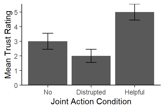
Figure 1. Mean levels of trust (1-7) by the three joint action conditions. Error bars are +/- 1 SE.

References

Demos, A.P., Carter, D.J., Wanderley, M.M., & Palmer, C (2017). The unresponsive partner: Roles of social status, auditory feedback, and animacy in coordination of joint music performance. Frontiers in Psychology, 149(8).

Demos, A.P., Chaffin, R., Begosh, K. T., Daniels, J. R., & Marsh, K. L. (2012). Rocking to the beat: Effects of music and partner’s movements on spontaneous interpersonal coordination. Journal of Experimental Psychology: General, 141(1), 49-53.

Hove, M. J., & Risen, J. L. (2009). It’s all in the timing: Interpersonal synchrony increases affiliation. Social cognition, 27(6), 949-960.

Launay, J., Dean, R. T., & Bailes, F. (2013). Synchronization can influence trust following virtual interaction. Experimental psychology, 60(1), 53-63.

Lenth, R. (2018). emmean: Estimated Marginal Means, aka Least-Squares Means. R Package Version 1.6.3. Available at: https://CRAN.R-project.org/package=emmeans.

Singmann, H., Bolker, B., Westfall, J., and Aust, F. (2021). afex: Analysis of Factorial Experiments. R Package Version 1.0-1. Available at: https://CRAN.R-project.org/package=afex.