Multi-Level Modeling: Three Levels
Designs
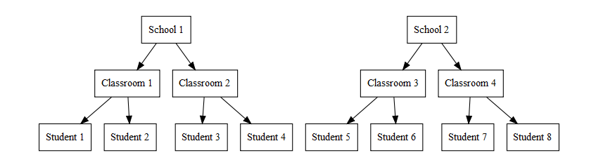
- 3 level models are used when you multiple levels of nesting that you
need to account for.
- Students nested in classrooms, nested in schools
- Patients nested in doctors, nested in hospitals
3 Levels
3 Level Model
Example
- Lets again examine active learning as it relates to math scores.
- You measure students math scores (DV) and the
proportion of time (IV) they spend using the computer
(which you assign)
- You expect that the more time they spend doing the active learning method, the higher their math test scores will be
- You collected data in many classrooms in three different schools.
- The number of classrooms can vary by schools, and the number of students per classroom can vary
- You think your system might work best for classrooms with a lot of students (you cannot control for that, but you know how many students are in each classroom)
- You measure students math scores (DV) and the
proportion of time (IV) they spend using the computer
(which you assign)
- Let’s go collect (simulate) our study (not shown here because of its length)
- Download Data
MLM.Data.L3<-read.csv("Mixed/Sim3level.csv")
# We need to set Classroom as a factor (since it was #)
MLM.Data.L3$Classroom.F<-as.factor(MLM.Data.L3$Classroom)
Sample Sizes
- Tabulate number of students per classroom per school
names(MLM.Data.L3)## [1] "Math" "ActiveTime" "ClassSize" "Classroom" "School"
## [6] "StudentID" "Classroom.F"CrossT <- table(MLM.Data.L3$School,MLM.Data.L3$Classroom.F)It seems that the data look somewhat balanced between schools, let’s just ignore the school-level (level 3)
Let’s just see the overall effect and ignore the classroom-level (level 2)
library(ggplot2)
library(gridExtra)

theme_set(theme_bw(base_size = 7, base_family = ""))

Active.Plot <-ggplot(data = MLM.Data.L3, aes(x = ActiveTime, y=Math))+
  coord_cartesian(ylim=c(10,80))+
  geom_point()+
  geom_smooth(method = "lm", se = TRUE)+
  xlab("Active Learning Time")+ylab("Math Score")+
  theme(legend.position = "none")

Size.Plot <-ggplot(data = MLM.Data.L3, aes(x = ClassSize, y=Math))+
  coord_cartesian(ylim=c(10,80))+
  geom_point()+
  geom_smooth(method = "lm", se = TRUE)+
  xlab("Class Size")+ylab("Math Score")+
  theme(legend.position = "top")

 grid.arrange(Size.Plot, Active.Plot, ncol=2)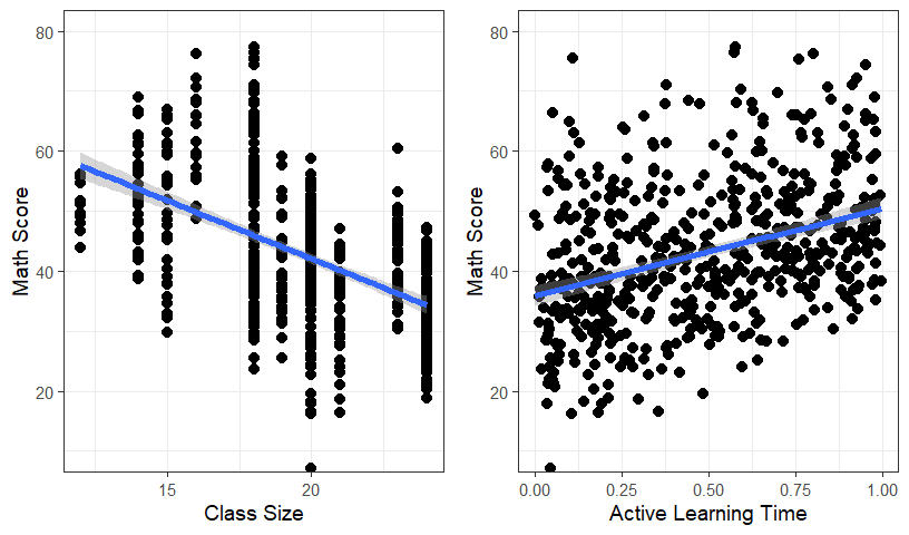
- Let’s just see: add in the classroom-level (level 2)
- But wait? Can we view Class size as a function of the classroom?
- No because each classroom only as 1 class size
library(ggplot2)
theme_set(theme_bw(base_size = 10, base_family = ""))

Active.Class <-ggplot(data = MLM.Data.L3, aes(x = ActiveTime, y=Math,group=Classroom.F))+
  coord_cartesian(ylim=c(10,80))+
  geom_point()+
  geom_smooth(method = "lm", se = TRUE, aes(colour = Classroom.F))+
  xlab("Active Learning Time")+ylab("Math Score")+
  theme(legend.position = "none")
Active.Class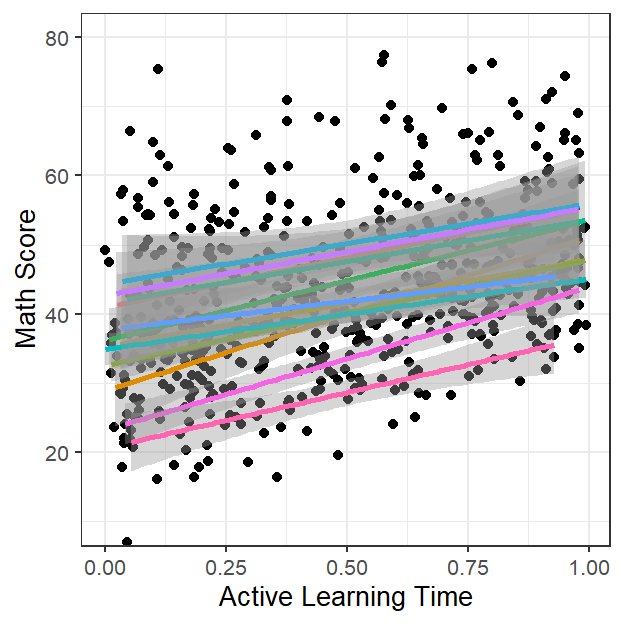
Recap 2-Level MLM
- Let’s ignore the school level and deal only as if this were 2 level MLM
- So students nested in classrooms
- Problem is we have multiple classrooms with the same number: we can fix that in R easily
MLM.Data.L3$Classroom.F2<-paste(MLM.Data.L3$School,MLM.Data.L3$Classroom.F,sep=":")Random intercept only Model
- Grand mean center
MLM.Data.L3$ActiveTime.GM<-scale(MLM.Data.L3$ActiveTime,scale=F)
MLM.Data.L3$ClassSize.GM<-scale(MLM.Data.L3$ClassSize,scale=F)- Let test our cluster
library(lme4)
Model.0<-lmer(Math ~ 1
              +(1|Classroom.F2),
              data=MLM.Data.L3, REML=FALSE)
summary(Model.0)
## Linear mixed model fit by maximum likelihood . t-tests use Satterthwaite's
## method [lmerModLmerTest]
## Formula: Math ~ 1 + (1 | Classroom.F2)
## Data: MLM.Data.L3
##
## AIC BIC logLik deviance df.resid
## 3805.7 3818.7 -1899.8 3799.7 567
##
## Scaled residuals:
## Min 1Q Median 3Q Max
## -3.5139 -0.6710 -0.0039 0.6477 2.7589
##
## Random effects:
## Groups Name Variance Std.Dev.
## Classroom.F2 (Intercept) 108.41 10.412
## Residual 37.22 6.101
## Number of obs: 570, groups: Classroom.F2, 30
##
## Fixed effects:
## Estimate Std. Error df t value Pr(>|t|)
## (Intercept) 43.990 1.919 29.977 22.93 <2e-16 ***
## ---
## Signif. codes: 0 '***' 0.001 '**' 0.01 '*' 0.05 '.' 0.1 ' ' 1- Check to make sure the cluster explains any variance
library(performance)
icc(Model.0)
## # Intraclass Correlation Coefficient
##
## Adjusted ICC: 0.744
## Unadjusted ICC: 0.744- Let test our fixed effects
Model.1<-lmer(Math ~ ActiveTime.GM+ClassSize.GM
              +(1|Classroom.F2),
              data=MLM.Data.L3, REML=FALSE)
summary(Model.1)
## Linear mixed model fit by maximum likelihood . t-tests use Satterthwaite's
## method [lmerModLmerTest]
## Formula: Math ~ ActiveTime.GM + ClassSize.GM + (1 | Classroom.F2)
## Data: MLM.Data.L3
##
## AIC BIC logLik deviance df.resid
## 3390.1 3411.9 -1690.1 3380.1 565
##
## Scaled residuals:
## Min 1Q Median 3Q Max
## -3.3148 -0.6516 -0.0386 0.6312 3.1178
##
## Random effects:
## Groups Name Variance Std.Dev.
## Classroom.F2 (Intercept) 72.29 8.503
## Residual 17.51 4.184
## Number of obs: 570, groups: Classroom.F2, 30
##
## Fixed effects:
## Estimate Std. Error df t value Pr(>|t|)
## (Intercept) 42.9594 1.5847 29.9349 27.109 < 2e-16 ***
## ActiveTime.GM 14.9403 0.6061 540.6478 24.651 < 2e-16 ***
## ClassSize.GM -1.8671 0.4802 30.0467 -3.888 0.000518 ***
## ---
## Signif. codes: 0 '***' 0.001 '**' 0.01 '*' 0.05 '.' 0.1 ' ' 1
##
## Correlation of Fixed Effects:
## (Intr) AcT.GM
## ActiveTm.GM 0.000
## ClassSiz.GM 0.167 0.001- So we have main effects. Lets check for the interaction
Model.2<-lmer(Math ~ ActiveTime.GM*ClassSize.GM
              +(1|Classroom.F2),
              data=MLM.Data.L3, REML=FALSE)
summary(Model.2)
## Linear mixed model fit by maximum likelihood . t-tests use Satterthwaite's
## method [lmerModLmerTest]
## Formula: Math ~ ActiveTime.GM * ClassSize.GM + (1 | Classroom.F2)
## Data: MLM.Data.L3
##
## AIC BIC logLik deviance df.resid
## 3388.7 3414.8 -1688.3 3376.7 564
##
## Scaled residuals:
## Min 1Q Median 3Q Max
## -3.3103 -0.6642 -0.0358 0.6455 3.1392
##
## Random effects:
## Groups Name Variance Std.Dev.
## Classroom.F2 (Intercept) 72.41 8.509
## Residual 17.40 4.171
## Number of obs: 570, groups: Classroom.F2, 30
##
## Fixed effects:
## Estimate Std. Error df t value Pr(>|t|)
## (Intercept) 42.9645 1.5858 29.9350 27.093 < 2e-16 ***
## ActiveTime.GM 14.9057 0.6044 540.6574 24.662 < 2e-16 ***
## ClassSize.GM -1.8662 0.4805 30.0457 -3.884 0.000524 ***
## ActiveTime.GM:ClassSize.GM 0.3613 0.1939 540.5862 1.863 0.062999 .
## ---
## Signif. codes: 0 '***' 0.001 '**' 0.01 '*' 0.05 '.' 0.1 ' ' 1
##
## Correlation of Fixed Effects:
## (Intr) AcT.GM ClS.GM
## ActiveTm.GM 0.000
## ClassSiz.GM 0.167 0.001
## AT.GM:CS.GM 0.002 -0.031 0.001- The interaction is weak, model testing will probably show the same result
anova(Model.1,Model.2)## Data: MLM.Data.L3
## Models:
## Model.1: Math ~ ActiveTime.GM + ClassSize.GM + (1 | Classroom.F2)
## Model.2: Math ~ ActiveTime.GM * ClassSize.GM + (1 | Classroom.F2)
## npar AIC BIC logLik deviance Chisq Df Pr(>Chisq)
## Model.1 5 3390.1 3411.9 -1690.1 3380.1
## Model.2 6 3388.7 3414.8 -1688.3 3376.7 3.4595 1 0.06289 .
## ---
## Signif. codes: 0 '***' 0.001 '**' 0.01 '*' 0.05 '.' 0.1 ' ' 1Plot Random slopes
- Lets plot the random and fixed effects (per classroom)
- First, we will
predictthe model results
MLM.Data.L3$Model.2.FR<-predict(Model.2, newdata=MLM.Data.L3)- Lets plot the raw data with the fitted of ActiveTime
theme_set(theme_bw(base_size = 7, base_family = ""))

Active.Class.School <-ggplot(data = MLM.Data.L3, aes(x = ActiveTime, y=Math,group=Classroom.F))+
  coord_cartesian(ylim=c(10,80))+
  geom_point(aes(colour = Classroom.F))+
  geom_smooth(method = "lm", se = TRUE, aes(colour = Classroom.F))+
  xlab("Active Learning Time")+ylab("Math Score")+
  theme(legend.position = "none")

Active.Class.School.fit <-ggplot(data = MLM.Data.L3, aes(x = ActiveTime, y=Model.2.FR,group=Classroom.F))+
  coord_cartesian(ylim=c(10,80))+
  geom_point(aes(colour = Classroom.F))+
  geom_smooth(method = "lm", se = TRUE, aes(colour = Classroom.F))+
  xlab("Active Learning Time")+ylab("Math Score - Model 2")+
  theme(legend.position = "none")

 grid.arrange(Active.Class.School, Active.Class.School.fit, ncol=2)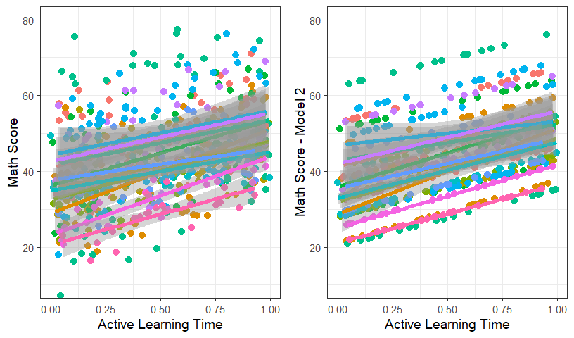
- Lets add random slopes to this final model and see that happens.
- There are alot of classrooms and we can see in the figure that the slopes do not have a lot of variance
Random Coefficients Model
- Lets add the level 1 slope (Activetime) as function of the classroom
Model.2.RC<-lmer(Math ~ ActiveTime.GM*ClassSize.GM
              +(1+ActiveTime.GM|Classroom.F2),
              data=MLM.Data.L3, REML=FALSE)
summary(Model.2.RC)
## Linear mixed model fit by maximum likelihood . t-tests use Satterthwaite's
## method [lmerModLmerTest]
## Formula:
## Math ~ ActiveTime.GM * ClassSize.GM + (1 + ActiveTime.GM | Classroom.F2)
## Data: MLM.Data.L3
##
## AIC BIC logLik deviance df.resid
## 3358.3 3393.1 -1671.1 3342.3 562
##
## Scaled residuals:
## Min 1Q Median 3Q Max
## -3.04260 -0.65433 -0.03363 0.63223 3.07726
##
## Random effects:
## Groups Name Variance Std.Dev. Corr
## Classroom.F2 (Intercept) 73.65 8.582
## ActiveTime.GM 22.19 4.711 -0.31
## Residual 15.34 3.916
## Number of obs: 570, groups: Classroom.F2, 30
##
## Fixed effects:
## Estimate Std. Error df t value Pr(>|t|)
## (Intercept) 42.8612 1.5984 29.9458 26.815 < 2e-16 ***
## ActiveTime.GM 14.8927 1.0450 30.3150 14.251 5.61e-15 ***
## ClassSize.GM -1.8703 0.4843 30.0394 -3.862 0.000556 ***
## ActiveTime.GM:ClassSize.GM 0.3329 0.3263 33.1054 1.020 0.315013
## ---
## Signif. codes: 0 '***' 0.001 '**' 0.01 '*' 0.05 '.' 0.1 ' ' 1
##
## Correlation of Fixed Effects:
## (Intr) AcT.GM ClS.GM
## ActiveTm.GM -0.258
## ClassSiz.GM 0.167 -0.043
## AT.GM:CS.GM -0.042 0.102 -0.250- The interaction disappeared but the pattern of the other variables held
- However, we are ignoring school-level variable. Lets re-plot our data see if we missed anything
Plotting 3 Levels
- There are many options on how to do this
- Since we have only three schools, lets try facet plotting
theme_set(theme_bw(base_size = 7, base_family = ""))

Active.Class.School <-ggplot(data = MLM.Data.L3, aes(x = ActiveTime, y=Math,group=Classroom.F))+
  facet_grid(~School)+
  coord_cartesian(ylim=c(10,80))+
  geom_point(aes(colour = Classroom.F))+
  geom_smooth(method = "lm", se = TRUE, aes(colour = Classroom.F))+
  xlab("Active Learning Time")+ylab("Math Score")+
  theme(legend.position = "none")

Size.School <-ggplot(data = MLM.Data.L3, aes(x = ClassSize, y=Math))+
  facet_grid(~School)+
  coord_cartesian(ylim=c(10,80))+
  geom_point()+
  geom_smooth(method = "lm", se = TRUE)+
  xlab("Class Size")+ylab("Math Score")+
  theme(legend.position = "top")

grid.arrange(Active.Class.School, Size.School, ncol=1, nrow=2)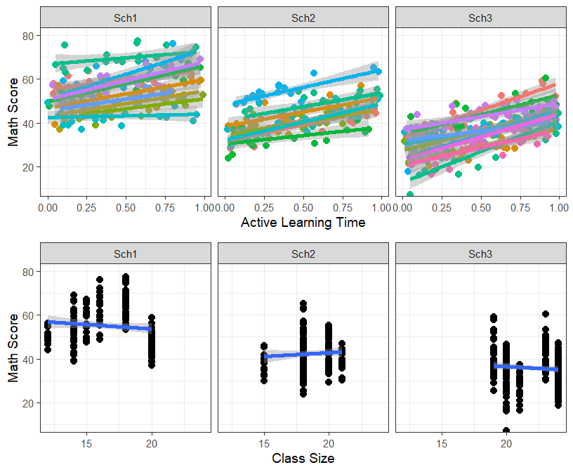
- We can also visualize it this way (by School)
library(dplyr)
Plot.Means<-MLM.Data.L3 %>% group_by(School) %>%
  dplyr::summarize(MathM=mean(Math, na.rm=TRUE),
           ClassSizeM=mean(ClassSize, na.rm=TRUE))

MathM.school<-ggplot(data = Plot.Means, aes(x = reorder(School, -MathM), y=MathM))+
  geom_point(aes(size = ClassSizeM))+
  xlab("")+ylab("Math Score")+
  theme_bw()+
  theme(legend.position = "top")
MathM.school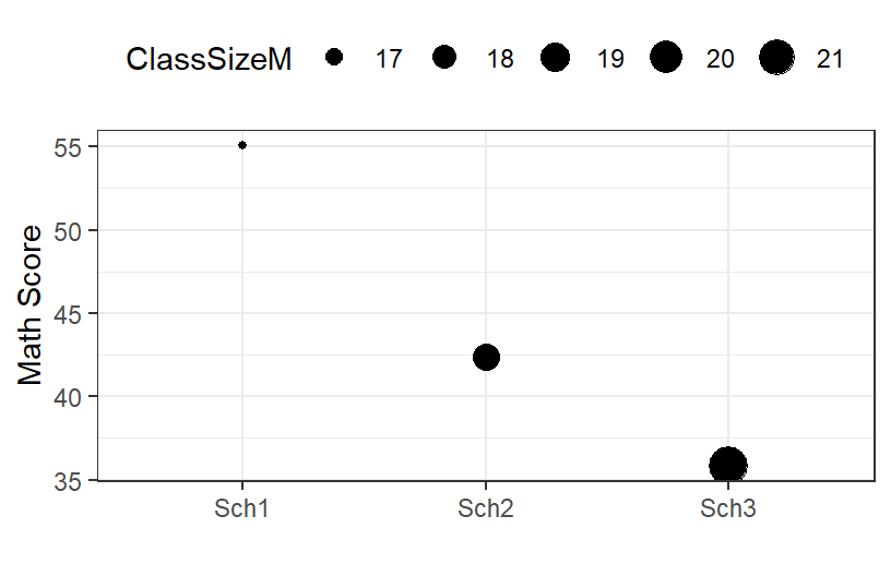
- You can see the size the dot changes as a function of the school!
- The school seems to make a huge difference
- The slope for Class Size seems to have vanished (Oh no, Simpson’s paradox again)
- We should control for school as a random intercept!
Confounded Variables
- It is clear from the figure for that Active learning spans the whole range for both classroom and school, but ClassSize is confounded
- Clearly the slopes vary a function of the school, but if we grand
mean centering ClassSize it will be confounded with the school
- In other words, ClassSize seems to vary as a function of the School if we test the fixed effect its going cross-over the schools (level 3 variable)
- So whatever fixed effect we find could mean that is a function of the school (level 3) or really something about the variable? We cannot know!
- So the only thing we do is center relative to the cluster
- This NOT the case for Active learning because we assigned subjects to that condition
- To make this variable meaningful lets re-center ClassSize based on School
- Note: This variable now means something new! It means, “how does class size affect math score, relative the school you are in
library(plyr)
# Level 3 Cluster mean
MLM.Data.L3<-ddply(MLM.Data.L3,.(School), mutate, CS.School.Mean = mean(ClassSize))
MLM.Data.L3$ClassSize.SC<-MLM.Data.L3$ClassSize-MLM.Data.L3$CS.School.Mean- See new plot
Size.School.2 <-ggplot(data = MLM.Data.L3, aes(x = ClassSize.SC, y=Math))+
  facet_grid(~School)+
  coord_cartesian(ylim=c(10,80))+
  geom_point()+
  geom_smooth(method = "lm", se = TRUE)+
  xlab("Class Size")+ylab("Math Score")+
  theme_bw()+
  theme(legend.position = "top")
Size.School.2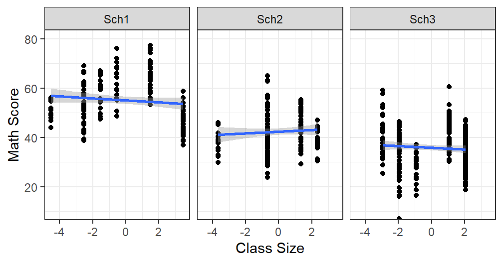
- Yes thats better, we removed the confound (but we need to be careful how we talk about it if we get any thing, but clearly from the graph we should not get much)
3 Level Random intercepts model
- We simply just need to add more random effects
+(1|School)= each school can have its own intercept+(1|School:Classroom.F)= each classroom can have its own intercept relative to which school its nested in- Note: I used
Classroom.Fand not our newClassroom.F2.Classroom.Fis not implicitly nested in classroom (there were multiple classroom 1), thus we must tell the function that classroom were nested in schoolsClassroom.F2is implicitly nested in classroom- Thus
+(1|School) + (1|School:Classroom.F)=+(1|School) + (1|Classroom.F2) - The results will be all the same!
library(lme4)
L3.Model.0<-lmer(Math ~ 1
              +(1|School)
              +(1|School:Classroom.F),
              data=MLM.Data.L3, REML=FALSE)
summary(L3.Model.0)
## Linear mixed model fit by maximum likelihood . t-tests use Satterthwaite's
## method [lmerModLmerTest]
## Formula: Math ~ 1 + (1 | School) + (1 | School:Classroom.F)
## Data: MLM.Data.L3
##
## AIC BIC logLik deviance df.resid
## 3789.8 3807.2 -1890.9 3781.8 566
##
## Scaled residuals:
## Min 1Q Median 3Q Max
## -3.5237 -0.6756 -0.0005 0.6546 2.7491
##
## Random effects:
## Groups Name Variance Std.Dev.
## School:Classroom.F (Intercept) 44.92 6.702
## School (Intercept) 59.88 7.738
## Residual 37.22 6.101
## Number of obs: 570, groups: School:Classroom.F, 30; School, 3
##
## Fixed effects:
## Estimate Std. Error df t value Pr(>|t|)
## (Intercept) 44.411 4.644 3.035 9.563 0.00231 **
## ---
## Signif. codes: 0 '***' 0.001 '**' 0.01 '*' 0.05 '.' 0.1 ' ' 1- Look at the random intercepts: Seems that school should not have been ignored
- Let verify via ICC
icc(L3.Model.0)## # Intraclass Correlation Coefficient
##
## Adjusted ICC: 0.738
## Unadjusted ICC: 0.738Clearly school level was important to explaining the data
Let’s check our main effects now.
- Class Size effect should go away based on what we saw in the graph!
L3.Model.1<-lmer(Math ~ ActiveTime.GM+ClassSize.SC
              +(1|School)
              +(1|School:Classroom.F),
              data=MLM.Data.L3, REML=FALSE)
summary(L3.Model.1)
## Linear mixed model fit by maximum likelihood . t-tests use Satterthwaite's
## method [lmerModLmerTest]
## Formula:
## Math ~ ActiveTime.GM + ClassSize.SC + (1 | School) + (1 | School:Classroom.F)
## Data: MLM.Data.L3
##
## AIC BIC logLik deviance df.resid
## 3385.9 3412.0 -1686.9 3373.9 564
##
## Scaled residuals:
## Min 1Q Median 3Q Max
## -3.3123 -0.6496 -0.0515 0.6336 3.0742
##
## Random effects:
## Groups Name Variance Std.Dev.
## School:Classroom.F (Intercept) 44.69 6.685
## School (Intercept) 60.42 7.773
## Residual 17.51 4.184
## Number of obs: 570, groups: School:Classroom.F, 30; School, 3
##
## Fixed effects:
## Estimate Std. Error df t value Pr(>|t|)
## (Intercept) 44.4402 4.6607 3.0415 9.535 0.00231 **
## ActiveTime.GM 14.9488 0.6060 540.9288 24.669 < 2e-16 ***
## ClassSize.SC -0.0306 0.5688 27.1017 -0.054 0.95749
## ---
## Signif. codes: 0 '***' 0.001 '**' 0.01 '*' 0.05 '.' 0.1 ' ' 1
##
## Correlation of Fixed Effects:
## (Intr) AcT.GM
## ActiveTm.GM 0.001
## ClassSiz.SC 0.031 0.007- Interaction could still be real, lets check:
L3.Model.2<-lmer(Math ~ ActiveTime.GM*ClassSize.SC
              +(1|School)
              +(1|School:Classroom.F),
              data=MLM.Data.L3, REML=FALSE)
summary(L3.Model.2)
## Linear mixed model fit by maximum likelihood . t-tests use Satterthwaite's
## method [lmerModLmerTest]
## Formula:
## Math ~ ActiveTime.GM * ClassSize.SC + (1 | School) + (1 | School:Classroom.F)
## Data: MLM.Data.L3
##
## AIC BIC logLik deviance df.resid
## 3379.9 3410.3 -1682.9 3365.9 563
##
## Scaled residuals:
## Min 1Q Median 3Q Max
## -3.13965 -0.62420 -0.01136 0.62253 2.84136
##
## Random effects:
## Groups Name Variance Std.Dev.
## School:Classroom.F (Intercept) 45.03 6.711
## School (Intercept) 60.36 7.769
## Residual 17.25 4.153
## Number of obs: 570, groups: School:Classroom.F, 30; School, 3
##
## Fixed effects:
## Estimate Std. Error df t value Pr(>|t|)
## (Intercept) 44.4184 4.6597 3.0422 9.532 0.00231 **
## ActiveTime.GM 14.9967 0.6017 540.9271 24.926 < 2e-16 ***
## ClassSize.SC -0.0368 0.5709 27.1003 -0.064 0.94908
## ActiveTime.GM:ClassSize.SC -0.8211 0.2893 540.8396 -2.839 0.00470 **
## ---
## Signif. codes: 0 '***' 0.001 '**' 0.01 '*' 0.05 '.' 0.1 ' ' 1
##
## Correlation of Fixed Effects:
## (Intr) AcT.GM ClS.SC
## ActiveTm.GM 0.000
## ClassSiz.SC 0.031 0.007
## AT.GM:CS.SC 0.002 -0.028 0.004- Significant interaction!
- But wait…
3 Level Random Coefficients model
Level 1 Random Slopes at Level 3
- Now let think this out for minute, we have level 1 slopes (ActiveTime) as a function of the classroom (level 2), but can they also vary as function of the school (level 3)?
- Lets look and see…
Active.School <-ggplot(data = MLM.Data.L3, aes(x = ActiveTime, y=Math, group=School))+
  geom_point(aes(color=School))+
  geom_smooth(method = "lm", se = TRUE,aes(color=School))+
  xlab("Active Learning Time")+ylab("Math Score")+
  theme_bw()+
  theme(legend.position = "none")
Active.School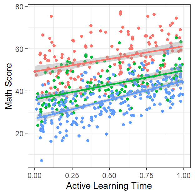
- With only our three schools it seems not really (slopes all look mostly the same).
- Also, the random slopes will perfectly correlate with the random intercepts!
- See below:
L3.Model.2a<-lmer(Math ~ ActiveTime.GM*ClassSize.SC
              +(1+ActiveTime.GM|School)
              +(1|School:Classroom.F),
              data=MLM.Data.L3, REML=FALSE)
summary(L3.Model.2a)
## Linear mixed model fit by maximum likelihood . t-tests use Satterthwaite's
## method [lmerModLmerTest]
## Formula: Math ~ ActiveTime.GM * ClassSize.SC + (1 + ActiveTime.GM | School) +
## (1 | School:Classroom.F)
## Data: MLM.Data.L3
##
## AIC BIC logLik deviance df.resid
## 3360.5 3399.6 -1671.2 3342.5 561
##
## Scaled residuals:
## Min 1Q Median 3Q Max
## -2.86601 -0.66736 -0.04249 0.64750 2.62037
##
## Random effects:
## Groups Name Variance Std.Dev. Corr
## School:Classroom.F (Intercept) 44.874 6.699
## School (Intercept) 60.076 7.751
## ActiveTime.GM 8.174 2.859 -1.00
## Residual 16.478 4.059
## Number of obs: 570, groups: School:Classroom.F, 30; School, 3
##
## Fixed effects:
## Estimate Std. Error df t value Pr(>|t|)
## (Intercept) 44.56614 4.64705 3.04601 9.590 0.00226 **
## ActiveTime.GM 14.35446 1.75474 3.07930 8.180 0.00347 **
## ClassSize.SC -0.04435 0.56933 27.83552 -0.078 0.93847
## ActiveTime.GM:ClassSize.SC -0.81809 0.28292 539.72042 -2.892 0.00399 **
## ---
## Signif. codes: 0 '***' 0.001 '**' 0.01 '*' 0.05 '.' 0.1 ' ' 1
##
## Correlation of Fixed Effects:
## (Intr) AcT.GM ClS.SC
## ActiveTm.GM -0.907
## ClassSiz.SC 0.031 0.001
## AT.GM:CS.SC 0.001 -0.008 0.004
## optimizer (nloptwrap) convergence code: 0 (OK)
## boundary (singular) fit: see help('isSingular')- We could remove the correlation can capture the slight differences in slope
L3.Model.2b<-lmer(Math ~ ActiveTime.GM*ClassSize.SC
              +(1+ActiveTime.GM||School)
              +(1|School:Classroom.F),
              data=MLM.Data.L3, REML=FALSE)
summary(L3.Model.2b)
## Linear mixed model fit by maximum likelihood . t-tests use Satterthwaite's
## method [lmerModLmerTest]
## Formula: Math ~ ActiveTime.GM * ClassSize.SC + (1 + ActiveTime.GM || School) +
## (1 | School:Classroom.F)
## Data: MLM.Data.L3
##
## AIC BIC logLik deviance df.resid
## 3364.2 3399.0 -1674.1 3348.2 562
##
## Scaled residuals:
## Min 1Q Median 3Q Max
## -2.8670 -0.6449 -0.0437 0.6589 2.5964
##
## Random effects:
## Groups Name Variance Std.Dev.
## School.Classroom.F (Intercept) 45.305 6.731
## School ActiveTime.GM 7.781 2.789
## School.1 (Intercept) 60.824 7.799
## Residual 16.492 4.061
## Number of obs: 570, groups: School:Classroom.F, 30; School, 3
##
## Fixed effects:
## Estimate Std. Error df t value Pr(>|t|)
## (Intercept) 44.3918 4.6772 3.0419 9.491 0.00234 **
## ActiveTime.GM 14.3027 1.7210 3.1071 8.311 0.00320 **
## ClassSize.SC -0.0287 0.5723 27.0995 -0.050 0.96037
## ActiveTime.GM:ClassSize.SC -0.8289 0.2831 538.1476 -2.928 0.00356 **
## ---
## Signif. codes: 0 '***' 0.001 '**' 0.01 '*' 0.05 '.' 0.1 ' ' 1
##
## Correlation of Fixed Effects:
## (Intr) AcT.GM ClS.SC
## ActiveTm.GM 0.000
## ClassSiz.SC 0.031 0.002
## AT.GM:CS.SC 0.002 -0.008 0.003Level 1 Random Slopes at Level 3 and Level 2
- However, is that variation a function of level 3 (school) is it really a function of level 2 (the classroom)
- Lets say its both and see what happens
L3.Model.2c<-lmer(Math ~ ActiveTime.GM*ClassSize.SC
              +(1+ActiveTime.GM||School)
              +(1+ActiveTime.GM|School:Classroom.F),
              data=MLM.Data.L3, REML=FALSE)
summary(L3.Model.2c)
## Linear mixed model fit by maximum likelihood . t-tests use Satterthwaite's
## method [lmerModLmerTest]
## Formula: Math ~ ActiveTime.GM * ClassSize.SC + (1 + ActiveTime.GM || School) +
## (1 + ActiveTime.GM | School:Classroom.F)
## Data: MLM.Data.L3
##
## AIC BIC logLik deviance df.resid
## 3353.0 3396.5 -1666.5 3333.0 560
##
## Scaled residuals:
## Min 1Q Median 3Q Max
## -3.01413 -0.62593 -0.04133 0.65070 2.84509
##
## Random effects:
## Groups Name Variance Std.Dev. Corr
## School.Classroom.F (Intercept) 46.143 6.793
## ActiveTime.GM 14.102 3.755 0.14
## School ActiveTime.GM 6.545 2.558
## School.1 (Intercept) 62.121 7.882
## Residual 15.326 3.915
## Number of obs: 570, groups: School:Classroom.F, 30; School, 3
##
## Fixed effects:
## Estimate Std. Error df t value Pr(>|t|)
## (Intercept) 44.35577 4.72608 3.03267 9.385 0.00245 **
## ActiveTime.GM 14.32683 1.73647 3.17701 8.251 0.00300 **
## ClassSize.SC -0.02766 0.57719 27.22576 -0.048 0.96213
## ActiveTime.GM:ClassSize.SC -0.77926 0.42308 29.96709 -1.842 0.07541 .
## ---
## Signif. codes: 0 '***' 0.001 '**' 0.01 '*' 0.05 '.' 0.1 ' ' 1
##
## Correlation of Fixed Effects:
## (Intr) AcT.GM ClS.SC
## ActiveTm.GM 0.015
## ClassSiz.SC 0.031 0.008
## AT.GM:CS.SC 0.004 0.027 0.104- Seems that maybe there is some variance at both we can capture.
- We lost the interaction: Seems that once we accounted for the random
slopes at Level 2 we lost the effect. Why?
- Remember each classroom had a different class size, adding variance to the slopes of ActiveTime.
- However, the model was explaining that variance via the fixed effect interaction between ActiveTime and Classsize. When we treated ActiveTime as random that fixed variance went the random slope (in this particular case. Do not think this generalizes to all datasets)
- Lets make sure we need all those random effects (run a LLT)
- Also lets check a simplier fit of the random random structure
L3.Model.2c<-lmer(Math ~ ActiveTime.GM*ClassSize.SC
              +(1+ActiveTime.GM||School)
              +(1+ActiveTime.GM|School:Classroom.F),
              data=MLM.Data.L3, REML=FALSE)

L3.Model.2c1<-lmer(Math ~ ActiveTime.GM*ClassSize.SC
              +(1|School)
              +(1+ActiveTime.GM|School:Classroom.F),
              data=MLM.Data.L3, REML=FALSE)
## Data: MLM.Data.L3
## Models:
## L3.Model.2: Math ~ ActiveTime.GM * ClassSize.SC + (1 | School) + (1 | School:Classroom.F)
## L3.Model.2b: Math ~ ActiveTime.GM * ClassSize.SC + (1 + ActiveTime.GM || School) + (1 | School:Classroom.F)
## L3.Model.2c: Math ~ ActiveTime.GM * ClassSize.SC + (1 + ActiveTime.GM || School) + (1 + ActiveTime.GM | School:Classroom.F)
## npar AIC BIC logLik deviance Chisq Df Pr(>Chisq)
## L3.Model.2 7 3379.9 3410.3 -1682.9 3365.9
## L3.Model.2b 8 3364.2 3399.0 -1674.1 3348.2 17.643 1 2.664e-05 ***
## L3.Model.2c 10 3353.0 3396.5 -1666.5 3333.0 15.205 2 0.0004993 ***
## ---
## Signif. codes: 0 '***' 0.001 '**' 0.01 '*' 0.05 '.' 0.1 ' ' 1## Data: MLM.Data.L3
## Models:
## L3.Model.2c1: Math ~ ActiveTime.GM * ClassSize.SC + (1 | School) + (1 + ActiveTime.GM | School:Classroom.F)
## L3.Model.2c: Math ~ ActiveTime.GM * ClassSize.SC + (1 + ActiveTime.GM || School) + (1 + ActiveTime.GM | School:Classroom.F)
## npar AIC BIC logLik deviance Chisq Df Pr(>Chisq)
## L3.Model.2c1 9 3354.8 3393.9 -1668.4 3336.8
## L3.Model.2c 10 3353.0 3396.5 -1666.5 3333.0 3.7377 1 0.0532 .
## ---
## Signif. codes: 0 '***' 0.001 '**' 0.01 '*' 0.05 '.' 0.1 ' ' 1- Seems that this random structure,
(1+ActiveTime.GM||School)+(1+ActiveTime.GM|School:Classroom.F)is marginally better than the simplier one,(1|School)+(1+ActiveTime.GM|School:Classroom.F). Which you use depends on your question. For now, lets use the more complex one for now
Plot Random Slopes
- Lets plot the random and fixed effects (per classroom) of our best fit model
- First, we will
predictthe model results
MLM.Data.L3$L3.Model.2c.FR<-predict(L3.Model.2c, newdata=MLM.Data.L3)- Lets plot the raw data with the fitted of ActiveTime
theme_set(theme_bw(base_size = 7, base_family = ""))

Active.Class.School <-ggplot(data = MLM.Data.L3,
                             aes(x = ActiveTime, y=Math,group=Classroom.F))+
  facet_grid(~School)+
  coord_cartesian(ylim=c(10,80))+
  geom_point(aes(colour = Classroom.F))+
  geom_smooth(method = "lm", se = TRUE, aes(colour = Classroom.F))+
  xlab("Active Learning Time")+ylab("Math Score")+
  theme(legend.position = "none")


Active.Class.School.Fit2c <-ggplot(data = MLM.Data.L3,
                             aes(x = ActiveTime, y=L3.Model.2c.FR, group=Classroom.F))+
  facet_grid(~School)+
  coord_cartesian(ylim=c(10,80))+
  geom_point(aes(colour = Classroom.F))+
  geom_smooth(method = "lm", se = TRUE, aes(colour = Classroom.F))+
  xlab("Active Learning Time")+ylab("Math Score - L3.Model.2c")+
  theme(legend.position = "none")

 grid.arrange(Active.Class.School, Active.Class.School.Fit2c, ncol=1, nrow=2)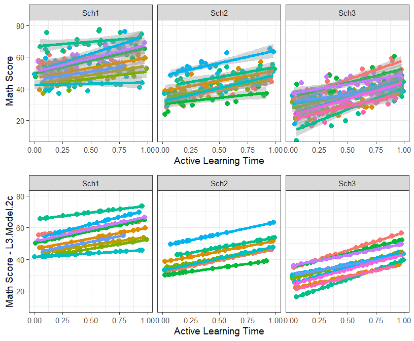
Level 2 Random Slopes at Level 3
- Are all the random issues we need to deal with?
- What do we do with Classsize, we saw earlier it seemed to vary a function of the classroom?
- It purely a level 2 slope and cannot vary as a function of the classroom, but it can vary a function of the school
- Lets remove all that ActiveTime and deal only with class size to understand what is going to happen
- Back to the figure and lets used our grand mean centered variable
Size.School.2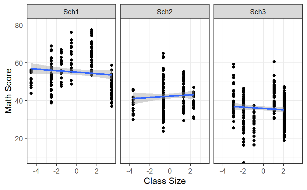
- Now we can test the slopes of ClassSize relative to School, but looking at the figure above, we already know the random intercept will correlate with the slope perfectly.
- Note: Normally when you have many level 3 (lots of schools) this will not always be true (or easy to visualize)
L3.Model.2d<-lmer(Math ~ ActiveTime.GM*ClassSize.SC
              +(1+ClassSize.SC|School)
              +(1|School:Classroom.F),
              data=MLM.Data.L3, REML=FALSE)
summary(L3.Model.2d, correlation=FALSE)
## Linear mixed model fit by maximum likelihood . t-tests use Satterthwaite's
## method [lmerModLmerTest]
## Formula: Math ~ ActiveTime.GM * ClassSize.SC + (1 + ClassSize.SC | School) +
## (1 | School:Classroom.F)
## Data: MLM.Data.L3
##
## AIC BIC logLik deviance df.resid
## 3383.9 3423.0 -1682.9 3365.9 561
##
## Scaled residuals:
## Min 1Q Median 3Q Max
## -3.13981 -0.62403 -0.01151 0.62256 2.84109
##
## Random effects:
## Groups Name Variance Std.Dev. Corr
## School:Classroom.F (Intercept) 4.503e+01 6.71051
## School (Intercept) 6.043e+01 7.77384
## ClassSize.SC 2.149e-04 0.01466 1.00
## Residual 1.725e+01 4.15279
## Number of obs: 570, groups: School:Classroom.F, 30; School, 3
##
## Fixed effects:
## Estimate Std. Error df t value Pr(>|t|)
## (Intercept) 44.41920 4.66234 3.03562 9.527 0.00234 **
## ActiveTime.GM 14.99664 0.60165 540.92818 24.926 < 2e-16 ***
## ClassSize.SC -0.03996 0.57091 27.07138 -0.070 0.94471
## ActiveTime.GM:ClassSize.SC -0.82110 0.28928 540.84064 -2.838 0.00470 **
## ---
## Signif. codes: 0 '***' 0.001 '**' 0.01 '*' 0.05 '.' 0.1 ' ' 1
## optimizer (nloptwrap) convergence code: 0 (OK)
## boundary (singular) fit: see help('isSingular')- Remove random slopes
L3.Model.2e<-lmer(Math ~ ActiveTime.GM*ClassSize.SC
              +(1+ClassSize.SC||School)
              +(1|School:Classroom.F),
              data=MLM.Data.L3, REML=FALSE)
summary(L3.Model.2e, correlation=FALSE)
## Linear mixed model fit by maximum likelihood . t-tests use Satterthwaite's
## method [lmerModLmerTest]
## Formula: Math ~ ActiveTime.GM * ClassSize.SC + (1 + ClassSize.SC || School) +
## (1 | School:Classroom.F)
## Data: MLM.Data.L3
##
## AIC BIC logLik deviance df.resid
## 3381.9 3416.7 -1682.9 3365.9 562
##
## Scaled residuals:
## Min 1Q Median 3Q Max
## -3.13965 -0.62420 -0.01136 0.62253 2.84136
##
## Random effects:
## Groups Name Variance Std.Dev.
## School.Classroom.F (Intercept) 45.03 6.711
## School ClassSize.SC 0.00 0.000
## School.1 (Intercept) 60.36 7.769
## Residual 17.25 4.153
## Number of obs: 570, groups: School:Classroom.F, 30; School, 3
##
## Fixed effects:
## Estimate Std. Error df t value Pr(>|t|)
## (Intercept) 44.4184 4.6597 3.0422 9.532 0.00231 **
## ActiveTime.GM 14.9967 0.6017 540.9271 24.926 < 2e-16 ***
## ClassSize.SC -0.0368 0.5709 27.1003 -0.064 0.94908
## ActiveTime.GM:ClassSize.SC -0.8211 0.2893 540.8396 -2.839 0.00470 **
## ---
## Signif. codes: 0 '***' 0.001 '**' 0.01 '*' 0.05 '.' 0.1 ' ' 1
## optimizer (nloptwrap) convergence code: 0 (OK)
## boundary (singular) fit: see help('isSingular')- Wait how did we get a zero random effect? Does this mean it has zero variance?
- We have few schools and only 3 slopes, and we are trying to test its fixed and random effects
- If we removed the fixed effects, the random slopes might appear
L3.Model.2f<-lmer(Math ~ ActiveTime.GM
              +(1+ClassSize.SC||School)
              +(1|School:Classroom.F),
              data=MLM.Data.L3, REML=FALSE)
summary(L3.Model.2f)
## Linear mixed model fit by maximum likelihood . t-tests use Satterthwaite's
## method [lmerModLmerTest]
## Formula:
## Math ~ ActiveTime.GM + (1 + ClassSize.SC || School) + (1 | School:Classroom.F)
## Data: MLM.Data.L3
##
## AIC BIC logLik deviance df.resid
## 3385.9 3412.0 -1686.9 3373.9 564
##
## Scaled residuals:
## Min 1Q Median 3Q Max
## -3.3121 -0.6498 -0.0517 0.6337 3.0737
##
## Random effects:
## Groups Name Variance Std.Dev.
## School.Classroom.F (Intercept) 44.69 6.685
## School ClassSize.SC 0.00 0.000
## School.1 (Intercept) 60.47 7.776
## Residual 17.51 4.184
## Number of obs: 570, groups: School:Classroom.F, 30; School, 3
##
## Fixed effects:
## Estimate Std. Error df t value Pr(>|t|)
## (Intercept) 44.448 4.660 3.037 9.537 0.00233 **
## ActiveTime.GM 14.949 0.606 540.983 24.670 < 2e-16 ***
## ---
## Signif. codes: 0 '***' 0.001 '**' 0.01 '*' 0.05 '.' 0.1 ' ' 1
##
## Correlation of Fixed Effects:
## (Intr)
## ActiveTm.GM 0.000
## optimizer (nloptwrap) convergence code: 0 (OK)
## boundary (singular) fit: see help('isSingular')- We got a number, but it is really small. Seems we should leave this level 2 random slope as fixed effect
Plot Final Results (Fixed effects only)
- Our best fit was L3.Model.2c
- Lets plot the interaction (but remember its tiny and not really significant)
library(effects)
# Set levels of support
SLevels<-c(mean(MLM.Data.L3$ClassSize.SC)-sd(MLM.Data.L3$ClassSize.SC),
                               mean(MLM.Data.L3$ClassSize.SC),
           mean(MLM.Data.L3$ClassSize.SC)+sd(MLM.Data.L3$ClassSize.SC))
#extract fixed effects
Results.BestFit<-Effect(c("ActiveTime.GM","ClassSize.SC"),L3.Model.2c,
     xlevels=list(ActiveTime.GM=seq(-.5,.5,.2),
                  ClassSize.SC=SLevels))
#Convert to data frame for ggplot
Results.BestFit<-as.data.frame(Results.BestFit)
#Label Support for graphing
Results.BestFit$ClassSize.F<-factor(Results.BestFit$ClassSize.SC,
                        levels=SLevels,
                         labels=c("Small Class", "Mean Class", "Large Class"))

#Plot fixed effect
Final.Fixed.Plot.1 <-ggplot(data = Results.BestFit,
                            aes(x = ActiveTime.GM, y =fit, group=ClassSize.F))+
  geom_line(size=2, aes(color=ClassSize.F,linetype=ClassSize.F))+
  coord_cartesian(xlim = c(-.5, .5),ylim = c(30, 60))+
  geom_ribbon(aes(ymin=fit-se, ymax=fit+se, group=ClassSize.F, fill=ClassSize.F),alpha=.2)+
  xlab("Proportion of Time Engaged in Active Learning \nCentered")+
  ylab("Math Score")+
  theme_bw()+
  theme(legend.position = "top",
        legend.title=element_blank())
Final.Fixed.Plot.1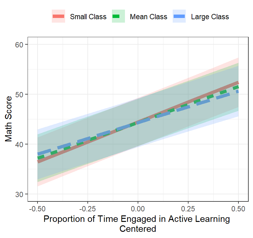
LS0tDQp0aXRsZTogJ011bHRpLUxldmVsIE1vZGVsaW5nOiBUaHJlZSBMZXZlbHMnDQpvdXRwdXQ6DQogIGh0bWxfZG9jdW1lbnQ6DQogICAgY29kZV9kb3dubG9hZDogeWVzDQogICAgZm9udHNpemU6IDhwdA0KICAgIGhpZ2hsaWdodDogdGV4dG1hdGUNCiAgICBudW1iZXJfc2VjdGlvbnM6IG5vDQogICAgdGhlbWU6IGZsYXRseQ0KICAgIHRvYzogeWVzDQogICAgdG9jX2Zsb2F0Og0KICAgICAgY29sbGFwc2VkOiBubw0KLS0tDQoNCmBgYHtyIHNldHVwLCBpbmNsdWRlPUZBTFNFfQ0Ka25pdHI6Om9wdHNfY2h1bmskc2V0KGNhY2hlPVRSVUUpDQprbml0cjo6b3B0c19jaHVuayRzZXQoZWNobyA9IFRSVUUpDQprbml0cjo6b3B0c19jaHVuayRzZXQobWVzc2FnZSA9IEZBTFNFKQ0Ka25pdHI6Om9wdHNfY2h1bmskc2V0KHdhcm5pbmcgPSAgRkFMU0UpDQprbml0cjo6b3B0c19jaHVuayRzZXQoZmlnLndpZHRoPTQuMjUpDQprbml0cjo6b3B0c19jaHVuayRzZXQoZmlnLmhlaWdodD00LjApDQprbml0cjo6b3B0c19jaHVuayRzZXQoZmlnLmFsaWduPSdjZW50ZXInKSANCmxpYnJhcnkoa25pdHIpDQpsaWJyYXJ5KGthYmxlRXh0cmEpDQpsaWJyYXJ5KGJyb29tLm1peGVkKQ0KYGBgDQoNCiMgRGVzaWducw0KLSAzIGxldmVsIG1vZGVscyBhcmUgdXNlZCB3aGVuIHlvdSBtdWx0aXBsZSBsZXZlbHMgb2YgbmVzdGluZyB0aGF0IHlvdSBuZWVkIHRvIGFjY291bnQgZm9yLg0KICAgIC0gU3R1ZGVudHMgbmVzdGVkIGluIGNsYXNzcm9vbXMsIG5lc3RlZCBpbiBzY2hvb2xzDQogICAgLSBQYXRpZW50cyBuZXN0ZWQgaW4gZG9jdG9ycywgbmVzdGVkIGluIGhvc3BpdGFscw0KDQojIDMgTGV2ZWxzIA0KDQohWzMgTGV2ZWwgTW9kZWxdKE1peGVkL0xldmVsMy5wbmcpDQoNCg0KIyMgRXhhbXBsZQ0KLSBMZXRzIGFnYWluIGV4YW1pbmUgYWN0aXZlIGxlYXJuaW5nIGFzIGl0IHJlbGF0ZXMgdG8gbWF0aCBzY29yZXMuIA0KICAgIC0gWW91IG1lYXN1cmUgc3R1ZGVudHMgKiptYXRoIHNjb3JlcyoqIChEVikgYW5kIHRoZSAqKnByb3BvcnRpb24gb2YgdGltZSoqIChJVikgdGhleSBzcGVuZCB1c2luZyB0aGUgY29tcHV0ZXIgKHdoaWNoIHlvdSBhc3NpZ24pDQogICAgICAgIC0gWW91IGV4cGVjdCB0aGF0IHRoZSBtb3JlIHRpbWUgdGhleSBzcGVuZCBkb2luZyB0aGUgYWN0aXZlIGxlYXJuaW5nIG1ldGhvZCwgdGhlIGhpZ2hlciB0aGVpciBtYXRoIHRlc3Qgc2NvcmVzIHdpbGwgYmUNCiAgICAtIFlvdSBjb2xsZWN0ZWQgZGF0YSBpbiBtYW55IGNsYXNzcm9vbXMgaW4gdGhyZWUgZGlmZmVyZW50IHNjaG9vbHMuIA0KICAgICAgICAtIFRoZSBudW1iZXIgb2YgY2xhc3Nyb29tcyBjYW4gdmFyeSBieSBzY2hvb2xzLCBhbmQgdGhlIG51bWJlciBvZiBzdHVkZW50cyBwZXIgY2xhc3Nyb29tIGNhbiB2YXJ5DQogICAgICAgIC0gWW91IHRoaW5rIHlvdXIgc3lzdGVtIG1pZ2h0IHdvcmsgYmVzdCBmb3IgY2xhc3Nyb29tcyB3aXRoIGEgbG90IG9mIHN0dWRlbnRzICh5b3UgY2Fubm90IGNvbnRyb2wgZm9yIHRoYXQsIGJ1dCB5b3Uga25vdyBob3cgbWFueSBzdHVkZW50cyBhcmUgaW4gZWFjaCBjbGFzc3Jvb20pDQotIExldCdzIGdvICpjb2xsZWN0KiAoc2ltdWxhdGUpIG91ciBzdHVkeSAobm90IHNob3duIGhlcmUgYmVjYXVzZSBvZiBpdHMgbGVuZ3RoKSANCi0gW0Rvd25sb2FkIERhdGFdKC9NaXhlZC9TaW0zbGV2ZWwuY3N2KQ0KDQpgYGB7cn0NCk1MTS5EYXRhLkwzPC1yZWFkLmNzdigiTWl4ZWQvU2ltM2xldmVsLmNzdiIpDQojIFdlIG5lZWQgdG8gc2V0IENsYXNzcm9vbSBhcyBhIGZhY3RvciAoc2luY2UgaXQgd2FzICMpDQpNTE0uRGF0YS5MMyRDbGFzc3Jvb20uRjwtYXMuZmFjdG9yKE1MTS5EYXRhLkwzJENsYXNzcm9vbSkNCmBgYA0KDQojIyMgU2FtcGxlIFNpemVzDQotIFRhYnVsYXRlIG51bWJlciBvZiBzdHVkZW50cyBwZXIgY2xhc3Nyb29tIHBlciBzY2hvb2wNCmBgYHtyfQ0KbmFtZXMoTUxNLkRhdGEuTDMpDQpDcm9zc1QgPC0gdGFibGUoTUxNLkRhdGEuTDMkU2Nob29sLE1MTS5EYXRhLkwzJENsYXNzcm9vbS5GKQ0KYGBgDQoNCmBgYHtyLCByZXN1bHRzPSdhc2lzJywgZWNobz1GQUxTRX0NCmxpYnJhcnkoa25pdHIpDQpsaWJyYXJ5KGthYmxlRXh0cmEpDQprYWJsZShDcm9zc1QsIGZvcm1hdD0ibGF0ZXgiKQ0KYGBgDQoNCi0gSXQgc2VlbXMgdGhhdCB0aGUgZGF0YSBsb29rICpzb21ld2hhdCogYmFsYW5jZWQgYmV0d2VlbiBzY2hvb2xzLCBsZXQncyBqdXN0IGlnbm9yZSB0aGUgc2Nob29sLWxldmVsIChsZXZlbCAzKQ0KDQotIExldCdzIGp1c3Qgc2VlIHRoZSBvdmVyYWxsIGVmZmVjdCBhbmQgaWdub3JlIHRoZSBjbGFzc3Jvb20tbGV2ZWwgKGxldmVsIDIpDQoNCmBgYHtyLCBvdXQud2lkdGggPSAnMTAwJScsIGZpZy5oZWlnaHQ9Mi41LCBmaWcuc2hvdz0naG9sZCcsZmlnLmFsaWduPSdjZW50ZXInfQ0KbGlicmFyeShnZ3Bsb3QyKQ0KbGlicmFyeShncmlkRXh0cmEpDQoNCnRoZW1lX3NldCh0aGVtZV9idyhiYXNlX3NpemUgPSA3LCBiYXNlX2ZhbWlseSA9ICIiKSkgDQoNCkFjdGl2ZS5QbG90IDwtZ2dwbG90KGRhdGEgPSBNTE0uRGF0YS5MMywgYWVzKHggPSBBY3RpdmVUaW1lLCB5PU1hdGgpKSsNCiAgY29vcmRfY2FydGVzaWFuKHlsaW09YygxMCw4MCkpKw0KICBnZW9tX3BvaW50KCkrDQogIGdlb21fc21vb3RoKG1ldGhvZCA9ICJsbSIsIHNlID0gVFJVRSkrDQogIHhsYWIoIkFjdGl2ZSBMZWFybmluZyBUaW1lIikreWxhYigiTWF0aCBTY29yZSIpKw0KICB0aGVtZShsZWdlbmQucG9zaXRpb24gPSAibm9uZSIpDQoNClNpemUuUGxvdCA8LWdncGxvdChkYXRhID0gTUxNLkRhdGEuTDMsIGFlcyh4ID0gQ2xhc3NTaXplLCB5PU1hdGgpKSsgIA0KICBjb29yZF9jYXJ0ZXNpYW4oeWxpbT1jKDEwLDgwKSkrDQogIGdlb21fcG9pbnQoKSsNCiAgZ2VvbV9zbW9vdGgobWV0aG9kID0gImxtIiwgc2UgPSBUUlVFKSsNCiAgeGxhYigiQ2xhc3MgU2l6ZSIpK3lsYWIoIk1hdGggU2NvcmUiKSsNCiAgdGhlbWUobGVnZW5kLnBvc2l0aW9uID0gInRvcCIpDQoNCiBncmlkLmFycmFuZ2UoU2l6ZS5QbG90LCBBY3RpdmUuUGxvdCwgbmNvbD0yKQ0KYGBgDQoNCi0gTGV0J3MganVzdCBzZWU6ICBhZGQgaW4gdGhlIGNsYXNzcm9vbS1sZXZlbCAobGV2ZWwgMikNCi0gQnV0IHdhaXQ/IENhbiB3ZSB2aWV3IENsYXNzIHNpemUgYXMgYSBmdW5jdGlvbiBvZiB0aGUgY2xhc3Nyb29tPyANCiAgICAtIE5vIGJlY2F1c2UgZWFjaCBjbGFzc3Jvb20gb25seSBhcyAxIGNsYXNzIHNpemUNCg0KYGBge3IsIGZpZy53aWR0aD0zLjI1LCBmaWcuaGVpZ2h0PTMuMjUsZmlnLnNob3c9J2hvbGQnLGZpZy5hbGlnbj0nY2VudGVyJ30NCmxpYnJhcnkoZ2dwbG90MikNCnRoZW1lX3NldCh0aGVtZV9idyhiYXNlX3NpemUgPSAxMCwgYmFzZV9mYW1pbHkgPSAiIikpIA0KDQpBY3RpdmUuQ2xhc3MgPC1nZ3Bsb3QoZGF0YSA9IE1MTS5EYXRhLkwzLCBhZXMoeCA9IEFjdGl2ZVRpbWUsIHk9TWF0aCxncm91cD1DbGFzc3Jvb20uRikpKw0KICBjb29yZF9jYXJ0ZXNpYW4oeWxpbT1jKDEwLDgwKSkrDQogIGdlb21fcG9pbnQoKSsNCiAgZ2VvbV9zbW9vdGgobWV0aG9kID0gImxtIiwgc2UgPSBUUlVFLCBhZXMoY29sb3VyID0gQ2xhc3Nyb29tLkYpKSsNCiAgeGxhYigiQWN0aXZlIExlYXJuaW5nIFRpbWUiKSt5bGFiKCJNYXRoIFNjb3JlIikrDQogIHRoZW1lKGxlZ2VuZC5wb3NpdGlvbiA9ICJub25lIikNCkFjdGl2ZS5DbGFzcw0KYGBgDQoNCiMgUmVjYXAgMi1MZXZlbCBNTE0NCi0gTGV0J3MgaWdub3JlIHRoZSBzY2hvb2wgbGV2ZWwgYW5kIGRlYWwgb25seSBhcyBpZiB0aGlzIHdlcmUgMiBsZXZlbCBNTE0gDQotIFNvIHN0dWRlbnRzIG5lc3RlZCBpbiBjbGFzc3Jvb21zDQotIFByb2JsZW0gaXMgd2UgaGF2ZSBtdWx0aXBsZSBjbGFzc3Jvb21zIHdpdGggdGhlIHNhbWUgbnVtYmVyOiB3ZSBjYW4gZml4IHRoYXQgaW4gUiBlYXNpbHkNCg0KYGBge3J9DQpNTE0uRGF0YS5MMyRDbGFzc3Jvb20uRjI8LXBhc3RlKE1MTS5EYXRhLkwzJFNjaG9vbCxNTE0uRGF0YS5MMyRDbGFzc3Jvb20uRixzZXA9IjoiKQ0KYGBgDQoNCiMjIFJhbmRvbSBpbnRlcmNlcHQgb25seSBNb2RlbA0KLSBHcmFuZCBtZWFuIGNlbnRlcg0KYGBge3J9DQpNTE0uRGF0YS5MMyRBY3RpdmVUaW1lLkdNPC1zY2FsZShNTE0uRGF0YS5MMyRBY3RpdmVUaW1lLHNjYWxlPUYpDQpNTE0uRGF0YS5MMyRDbGFzc1NpemUuR008LXNjYWxlKE1MTS5EYXRhLkwzJENsYXNzU2l6ZSxzY2FsZT1GKQ0KYGBgDQoNCi0gTGV0IHRlc3Qgb3VyIGNsdXN0ZXINCmBgYHtyfQ0KbGlicmFyeShsbWU0KQ0KTW9kZWwuMDwtbG1lcihNYXRoIH4gMQ0KICAgICAgICAgICAgICArKDF8Q2xhc3Nyb29tLkYyKSwgIA0KICAgICAgICAgICAgICBkYXRhPU1MTS5EYXRhLkwzLCBSRU1MPUZBTFNFKQ0Kc3VtbWFyeShNb2RlbC4wKQ0KYGBgDQotIENoZWNrIHRvIG1ha2Ugc3VyZSB0aGUgY2x1c3RlciBleHBsYWlucyBhbnkgdmFyaWFuY2UNCmBgYHtyfQ0KbGlicmFyeShwZXJmb3JtYW5jZSkNCmljYyhNb2RlbC4wKQ0KYGBgDQoNCi0gTGV0IHRlc3Qgb3VyIGZpeGVkIGVmZmVjdHMgDQoNCmBgYHtyfQ0KTW9kZWwuMTwtbG1lcihNYXRoIH4gQWN0aXZlVGltZS5HTStDbGFzc1NpemUuR00NCiAgICAgICAgICAgICAgKygxfENsYXNzcm9vbS5GMiksICANCiAgICAgICAgICAgICAgZGF0YT1NTE0uRGF0YS5MMywgUkVNTD1GQUxTRSkNCnN1bW1hcnkoTW9kZWwuMSkNCmBgYA0KDQotIFNvIHdlIGhhdmUgbWFpbiBlZmZlY3RzLiBMZXRzIGNoZWNrIGZvciB0aGUgaW50ZXJhY3Rpb24NCiAgDQpgYGB7cn0NCk1vZGVsLjI8LWxtZXIoTWF0aCB+IEFjdGl2ZVRpbWUuR00qQ2xhc3NTaXplLkdNDQogICAgICAgICAgICAgICsoMXxDbGFzc3Jvb20uRjIpLCAgDQogICAgICAgICAgICAgIGRhdGE9TUxNLkRhdGEuTDMsIFJFTUw9RkFMU0UpDQpzdW1tYXJ5KE1vZGVsLjIpDQpgYGANCi0gVGhlIGludGVyYWN0aW9uIGlzIHdlYWssIG1vZGVsIHRlc3Rpbmcgd2lsbCBwcm9iYWJseSBzaG93IHRoZSBzYW1lIHJlc3VsdCAgICANCmBgYHtyfQ0KYW5vdmEoTW9kZWwuMSxNb2RlbC4yKQ0KYGBgDQoNCiMjIyBQbG90IFJhbmRvbSBzbG9wZXMNCi0gTGV0cyBwbG90IHRoZSByYW5kb20gYW5kIGZpeGVkIGVmZmVjdHMgKHBlciBjbGFzc3Jvb20pDQotIEZpcnN0LCB3ZSB3aWxsIGBwcmVkaWN0YCB0aGUgbW9kZWwgcmVzdWx0cw0KYGBge3J9DQpNTE0uRGF0YS5MMyRNb2RlbC4yLkZSPC1wcmVkaWN0KE1vZGVsLjIsIG5ld2RhdGE9TUxNLkRhdGEuTDMpDQpgYGANCg0KLSBMZXRzIHBsb3QgdGhlIHJhdyBkYXRhIHdpdGggdGhlIGZpdHRlZCBvZiBBY3RpdmVUaW1lDQoNCmBgYHtyLCBvdXQud2lkdGggPSAnMTAwJScsIGZpZy5oZWlnaHQ9Mi41LCBmaWcuc2hvdz0naG9sZCcsZmlnLmFsaWduPSdjZW50ZXInfQ0KdGhlbWVfc2V0KHRoZW1lX2J3KGJhc2Vfc2l6ZSA9IDcsIGJhc2VfZmFtaWx5ID0gIiIpKSANCg0KQWN0aXZlLkNsYXNzLlNjaG9vbCA8LWdncGxvdChkYXRhID0gTUxNLkRhdGEuTDMsIGFlcyh4ID0gQWN0aXZlVGltZSwgeT1NYXRoLGdyb3VwPUNsYXNzcm9vbS5GKSkrDQogIGNvb3JkX2NhcnRlc2lhbih5bGltPWMoMTAsODApKSsNCiAgZ2VvbV9wb2ludChhZXMoY29sb3VyID0gQ2xhc3Nyb29tLkYpKSsNCiAgZ2VvbV9zbW9vdGgobWV0aG9kID0gImxtIiwgc2UgPSBUUlVFLCBhZXMoY29sb3VyID0gQ2xhc3Nyb29tLkYpKSsNCiAgeGxhYigiQWN0aXZlIExlYXJuaW5nIFRpbWUiKSt5bGFiKCJNYXRoIFNjb3JlIikrDQogIHRoZW1lKGxlZ2VuZC5wb3NpdGlvbiA9ICJub25lIikNCg0KQWN0aXZlLkNsYXNzLlNjaG9vbC5maXQgPC1nZ3Bsb3QoZGF0YSA9IE1MTS5EYXRhLkwzLCBhZXMoeCA9IEFjdGl2ZVRpbWUsIHk9TW9kZWwuMi5GUixncm91cD1DbGFzc3Jvb20uRikpKw0KICBjb29yZF9jYXJ0ZXNpYW4oeWxpbT1jKDEwLDgwKSkrDQogIGdlb21fcG9pbnQoYWVzKGNvbG91ciA9IENsYXNzcm9vbS5GKSkrDQogIGdlb21fc21vb3RoKG1ldGhvZCA9ICJsbSIsIHNlID0gVFJVRSwgYWVzKGNvbG91ciA9IENsYXNzcm9vbS5GKSkrDQogIHhsYWIoIkFjdGl2ZSBMZWFybmluZyBUaW1lIikreWxhYigiTWF0aCBTY29yZSAtIE1vZGVsIDIiKSsNCiAgdGhlbWUobGVnZW5kLnBvc2l0aW9uID0gIm5vbmUiKQ0KDQogZ3JpZC5hcnJhbmdlKEFjdGl2ZS5DbGFzcy5TY2hvb2wsIEFjdGl2ZS5DbGFzcy5TY2hvb2wuZml0LCBuY29sPTIpDQpgYGANCg0KLSBMZXRzIGFkZCByYW5kb20gc2xvcGVzIHRvIHRoaXMgZmluYWwgbW9kZWwgYW5kIHNlZSB0aGF0IGhhcHBlbnMuIA0KLSBUaGVyZSBhcmUgYWxvdCBvZiBjbGFzc3Jvb21zIGFuZCB3ZSBjYW4gc2VlIGluIHRoZSBmaWd1cmUgdGhhdCB0aGUgc2xvcGVzIGRvIG5vdCBoYXZlIGEgbG90IG9mIHZhcmlhbmNlDQoNCiMjIFJhbmRvbSBDb2VmZmljaWVudHMgTW9kZWwNCi0gTGV0cyBhZGQgdGhlIGxldmVsIDEgc2xvcGUgKEFjdGl2ZXRpbWUpIGFzIGZ1bmN0aW9uIG9mIHRoZSBjbGFzc3Jvb20NCg0KYGBge3J9DQpNb2RlbC4yLlJDPC1sbWVyKE1hdGggfiBBY3RpdmVUaW1lLkdNKkNsYXNzU2l6ZS5HTQ0KICAgICAgICAgICAgICArKDErQWN0aXZlVGltZS5HTXxDbGFzc3Jvb20uRjIpLCAgDQogICAgICAgICAgICAgIGRhdGE9TUxNLkRhdGEuTDMsIFJFTUw9RkFMU0UpDQpzdW1tYXJ5KE1vZGVsLjIuUkMpDQpgYGANCg0KLSBUaGUgaW50ZXJhY3Rpb24gZGlzYXBwZWFyZWQgYnV0IHRoZSBwYXR0ZXJuIG9mIHRoZSBvdGhlciB2YXJpYWJsZXMgaGVsZA0KLSBIb3dldmVyLCB3ZSBhcmUgaWdub3Jpbmcgc2Nob29sLWxldmVsIHZhcmlhYmxlLiBMZXRzIHJlLXBsb3Qgb3VyIGRhdGEgc2VlIGlmIHdlIG1pc3NlZCBhbnl0aGluZw0KDQojIFBsb3R0aW5nIDMgTGV2ZWxzDQotIFRoZXJlIGFyZSBtYW55IG9wdGlvbnMgb24gaG93IHRvIGRvIHRoaXMNCi0gU2luY2Ugd2UgaGF2ZSBvbmx5IHRocmVlIHNjaG9vbHMsIGxldHMgdHJ5IGZhY2V0IHBsb3R0aW5nDQoNCmBgYHtyLCBvdXQud2lkdGggPSAnNzUlJywgZmlnLmhlaWdodD0zLjUsIGZpZy5zaG93PSdob2xkJyxmaWcuYWxpZ249J2NlbnRlcid9DQoNCnRoZW1lX3NldCh0aGVtZV9idyhiYXNlX3NpemUgPSA3LCBiYXNlX2ZhbWlseSA9ICIiKSkgDQoNCkFjdGl2ZS5DbGFzcy5TY2hvb2wgPC1nZ3Bsb3QoZGF0YSA9IE1MTS5EYXRhLkwzLCBhZXMoeCA9IEFjdGl2ZVRpbWUsIHk9TWF0aCxncm91cD1DbGFzc3Jvb20uRikpKw0KICBmYWNldF9ncmlkKH5TY2hvb2wpKw0KICBjb29yZF9jYXJ0ZXNpYW4oeWxpbT1jKDEwLDgwKSkrDQogIGdlb21fcG9pbnQoYWVzKGNvbG91ciA9IENsYXNzcm9vbS5GKSkrDQogIGdlb21fc21vb3RoKG1ldGhvZCA9ICJsbSIsIHNlID0gVFJVRSwgYWVzKGNvbG91ciA9IENsYXNzcm9vbS5GKSkrDQogIHhsYWIoIkFjdGl2ZSBMZWFybmluZyBUaW1lIikreWxhYigiTWF0aCBTY29yZSIpKw0KICB0aGVtZShsZWdlbmQucG9zaXRpb24gPSAibm9uZSIpDQoNClNpemUuU2Nob29sIDwtZ2dwbG90KGRhdGEgPSBNTE0uRGF0YS5MMywgYWVzKHggPSBDbGFzc1NpemUsIHk9TWF0aCkpKw0KICBmYWNldF9ncmlkKH5TY2hvb2wpKw0KICBjb29yZF9jYXJ0ZXNpYW4oeWxpbT1jKDEwLDgwKSkrDQogIGdlb21fcG9pbnQoKSsNCiAgZ2VvbV9zbW9vdGgobWV0aG9kID0gImxtIiwgc2UgPSBUUlVFKSsNCiAgeGxhYigiQ2xhc3MgU2l6ZSIpK3lsYWIoIk1hdGggU2NvcmUiKSsNCiAgdGhlbWUobGVnZW5kLnBvc2l0aW9uID0gInRvcCIpDQoNCmdyaWQuYXJyYW5nZShBY3RpdmUuQ2xhc3MuU2Nob29sLCBTaXplLlNjaG9vbCwgbmNvbD0xLCBucm93PTIpDQpgYGANCg0KLSBXZSBjYW4gYWxzbyB2aXN1YWxpemUgaXQgdGhpcyB3YXkgKGJ5IFNjaG9vbCkNCg0KYGBge3IsIGZpZy53aWR0aD00LjI1LCBmaWcuaGVpZ2h0PTIuNzUsZmlnLnNob3c9J2hvbGQnLGZpZy5hbGlnbj0nY2VudGVyJ30NCmxpYnJhcnkoZHBseXIpDQpQbG90Lk1lYW5zPC1NTE0uRGF0YS5MMyAlPiUgZ3JvdXBfYnkoU2Nob29sKSAlPiUgIA0KICBkcGx5cjo6c3VtbWFyaXplKE1hdGhNPW1lYW4oTWF0aCwgbmEucm09VFJVRSksDQogICAgICAgICAgIENsYXNzU2l6ZU09bWVhbihDbGFzc1NpemUsIG5hLnJtPVRSVUUpKQ0KDQpNYXRoTS5zY2hvb2w8LWdncGxvdChkYXRhID0gUGxvdC5NZWFucywgYWVzKHggPSByZW9yZGVyKFNjaG9vbCwgLU1hdGhNKSwgeT1NYXRoTSkpKw0KICBnZW9tX3BvaW50KGFlcyhzaXplID0gQ2xhc3NTaXplTSkpKw0KICB4bGFiKCIiKSt5bGFiKCJNYXRoIFNjb3JlIikrDQogIHRoZW1lX2J3KCkrDQogIHRoZW1lKGxlZ2VuZC5wb3NpdGlvbiA9ICJ0b3AiKQ0KTWF0aE0uc2Nob29sDQpgYGANCg0KLSBZb3UgY2FuIHNlZSB0aGUgc2l6ZSB0aGUgZG90IGNoYW5nZXMgYXMgYSBmdW5jdGlvbiBvZiB0aGUgc2Nob29sIQ0KLSBUaGUgc2Nob29sIHNlZW1zIHRvIG1ha2UgYSBodWdlIGRpZmZlcmVuY2UNCi0gVGhlIHNsb3BlIGZvciBDbGFzcyBTaXplIHNlZW1zIHRvIGhhdmUgdmFuaXNoZWQgKE9oIG5vLCBTaW1wc29uJ3MgcGFyYWRveCBhZ2FpbikNCi0gV2Ugc2hvdWxkIGNvbnRyb2wgZm9yIHNjaG9vbCBhcyBhIHJhbmRvbSBpbnRlcmNlcHQhDQoNCiMjIENvbmZvdW5kZWQgVmFyaWFibGVzDQotIEl0IGlzIGNsZWFyIGZyb20gdGhlIGZpZ3VyZSBmb3IgdGhhdCBBY3RpdmUgbGVhcm5pbmcgc3BhbnMgdGhlIHdob2xlIHJhbmdlIGZvciBib3RoIGNsYXNzcm9vbSBhbmQgc2Nob29sLCBidXQgQ2xhc3NTaXplIGlzIGNvbmZvdW5kZWQNCi0gQ2xlYXJseSB0aGUgc2xvcGVzIHZhcnkgYSBmdW5jdGlvbiBvZiB0aGUgc2Nob29sLCBidXQgaWYgd2UgZ3JhbmQgbWVhbiBjZW50ZXJpbmcgQ2xhc3NTaXplIGl0IHdpbGwgYmUgY29uZm91bmRlZCB3aXRoIHRoZSBzY2hvb2wNCiAgICAtIEluIG90aGVyIHdvcmRzLCBDbGFzc1NpemUgc2VlbXMgdG8gdmFyeSBhcyBhIGZ1bmN0aW9uIG9mIHRoZSBTY2hvb2wgaWYgd2UgdGVzdCB0aGUgZml4ZWQgZWZmZWN0IGl0cyBnb2luZyBjcm9zcy1vdmVyIHRoZSBzY2hvb2xzIChsZXZlbCAzIHZhcmlhYmxlKQ0KICAgIC0gU28gd2hhdGV2ZXIgZml4ZWQgZWZmZWN0IHdlIGZpbmQgY291bGQgbWVhbiB0aGF0IGlzIGEgZnVuY3Rpb24gb2YgdGhlIHNjaG9vbCAobGV2ZWwgMykgb3IgcmVhbGx5IHNvbWV0aGluZyBhYm91dCB0aGUgdmFyaWFibGU/IFdlIGNhbm5vdCBrbm93ISANCiAgICAtIFNvIHRoZSBvbmx5IHRoaW5nIHdlIGRvIGlzIGNlbnRlciByZWxhdGl2ZSB0byB0aGUgY2x1c3Rlcg0KICAgIC0gKlRoaXMgTk9UIHRoZSBjYXNlIGZvciBBY3RpdmUgbGVhcm5pbmcgYmVjYXVzZSB3ZSBhc3NpZ25lZCBzdWJqZWN0cyB0byB0aGF0IGNvbmRpdGlvbioNCi0gVG8gbWFrZSB0aGlzIHZhcmlhYmxlIG1lYW5pbmdmdWwgbGV0cyByZS1jZW50ZXIgQ2xhc3NTaXplIGJhc2VkIG9uIFNjaG9vbA0KLSAqKk5vdGU6IFRoaXMgdmFyaWFibGUgbm93IG1lYW5zIHNvbWV0aGluZyBuZXchIEl0IG1lYW5zLCAiaG93IGRvZXMgY2xhc3Mgc2l6ZSBhZmZlY3QgbWF0aCBzY29yZSwgcmVsYXRpdmUgdGhlIHNjaG9vbCB5b3UgYXJlIGluKiogDQogDQoNCmBgYHtyfQ0KbGlicmFyeShwbHlyKQ0KIyBMZXZlbCAzIENsdXN0ZXIgbWVhbg0KTUxNLkRhdGEuTDM8LWRkcGx5KE1MTS5EYXRhLkwzLC4oU2Nob29sKSwgbXV0YXRlLCBDUy5TY2hvb2wuTWVhbiA9IG1lYW4oQ2xhc3NTaXplKSkNCk1MTS5EYXRhLkwzJENsYXNzU2l6ZS5TQzwtTUxNLkRhdGEuTDMkQ2xhc3NTaXplLU1MTS5EYXRhLkwzJENTLlNjaG9vbC5NZWFuDQpgYGANCg0KLSBTZWUgbmV3IHBsb3QNCg0KYGBge3IsIGZpZy53aWR0aD01LjI1LCBmaWcuaGVpZ2h0PTIuNzUsZmlnLnNob3c9J2hvbGQnLGZpZy5hbGlnbj0nY2VudGVyJ30NClNpemUuU2Nob29sLjIgPC1nZ3Bsb3QoZGF0YSA9IE1MTS5EYXRhLkwzLCBhZXMoeCA9IENsYXNzU2l6ZS5TQywgeT1NYXRoKSkrDQogIGZhY2V0X2dyaWQoflNjaG9vbCkrDQogIGNvb3JkX2NhcnRlc2lhbih5bGltPWMoMTAsODApKSsNCiAgZ2VvbV9wb2ludCgpKw0KICBnZW9tX3Ntb290aChtZXRob2QgPSAibG0iLCBzZSA9IFRSVUUpKw0KICB4bGFiKCJDbGFzcyBTaXplIikreWxhYigiTWF0aCBTY29yZSIpKw0KICB0aGVtZV9idygpKw0KICB0aGVtZShsZWdlbmQucG9zaXRpb24gPSAidG9wIikNClNpemUuU2Nob29sLjINCmBgYA0KDQotIFllcyB0aGF0cyBiZXR0ZXIsIHdlIHJlbW92ZWQgdGhlIGNvbmZvdW5kIChidXQgd2UgbmVlZCB0byBiZSBjYXJlZnVsIGhvdyB3ZSB0YWxrIGFib3V0IGl0IGlmIHdlIGdldCBhbnkgdGhpbmcsIGJ1dCBjbGVhcmx5IGZyb20gdGhlIGdyYXBoIHdlIHNob3VsZCBub3QgZ2V0IG11Y2gpDQoNCiMjIDMgTGV2ZWwgUmFuZG9tIGludGVyY2VwdHMgbW9kZWwNCi0gV2Ugc2ltcGx5IGp1c3QgbmVlZCB0byBhZGQgbW9yZSByYW5kb20gZWZmZWN0cw0KICAgIC0gYCsoMXxTY2hvb2wpYCA9IGVhY2ggc2Nob29sIGNhbiBoYXZlIGl0cyBvd24gaW50ZXJjZXB0DQogICAgLSBgKygxfFNjaG9vbDpDbGFzc3Jvb20uRilgID0gZWFjaCBjbGFzc3Jvb20gY2FuIGhhdmUgaXRzIG93biBpbnRlcmNlcHQgcmVsYXRpdmUgdG8gd2hpY2ggc2Nob29sIGl0cyBuZXN0ZWQgaW4NCiAgICAtIE5vdGU6IEkgdXNlZCBgQ2xhc3Nyb29tLkZgIGFuZCBub3Qgb3VyIG5ldyBgQ2xhc3Nyb29tLkYyYC4gDQogICAgICAgIC0gYENsYXNzcm9vbS5GYCBpcyBub3QgaW1wbGljaXRseSBuZXN0ZWQgaW4gY2xhc3Nyb29tICh0aGVyZSB3ZXJlIG11bHRpcGxlIGNsYXNzcm9vbSAxKSwgdGh1cyB3ZSBtdXN0IHRlbGwgdGhlIGZ1bmN0aW9uIHRoYXQgY2xhc3Nyb29tIHdlcmUgbmVzdGVkIGluIHNjaG9vbHMNCiAgICAgICAgLSBgQ2xhc3Nyb29tLkYyYGlzIGltcGxpY2l0bHkgbmVzdGVkIGluIGNsYXNzcm9vbSANCiAgICAgICAgLSBUaHVzIGArKDF8U2Nob29sKSArICgxfFNjaG9vbDpDbGFzc3Jvb20uRilgID0gYCsoMXxTY2hvb2wpICsgKDF8Q2xhc3Nyb29tLkYyKWANCiAgICAgICAgLSBUaGUgcmVzdWx0cyB3aWxsIGJlIGFsbCB0aGUgc2FtZSENCiAgICAgICAgDQpgYGB7cn0NCmxpYnJhcnkobG1lNCkNCkwzLk1vZGVsLjA8LWxtZXIoTWF0aCB+IDENCiAgICAgICAgICAgICAgKygxfFNjaG9vbCkNCiAgICAgICAgICAgICAgKygxfFNjaG9vbDpDbGFzc3Jvb20uRiksICANCiAgICAgICAgICAgICAgZGF0YT1NTE0uRGF0YS5MMywgUkVNTD1GQUxTRSkNCnN1bW1hcnkoTDMuTW9kZWwuMCkNCmBgYA0KDQotIExvb2sgYXQgdGhlIHJhbmRvbSBpbnRlcmNlcHRzOiBTZWVtcyB0aGF0IHNjaG9vbCBzaG91bGQgbm90IGhhdmUgYmVlbiBpZ25vcmVkDQotIExldCB2ZXJpZnkgdmlhIElDQw0KDQpgYGB7cn0NCmljYyhMMy5Nb2RlbC4wKQ0KYGBgDQoNCi0gQ2xlYXJseSBzY2hvb2wgbGV2ZWwgd2FzIGltcG9ydGFudCB0byBleHBsYWluaW5nIHRoZSBkYXRhDQoNCi0gTGV0J3MgY2hlY2sgb3VyIG1haW4gZWZmZWN0cyBub3cuIA0KICAgIC0gQ2xhc3MgU2l6ZSBlZmZlY3Qgc2hvdWxkIGdvIGF3YXkgYmFzZWQgb24gd2hhdCB3ZSBzYXcgaW4gdGhlIGdyYXBoIQ0KICAgIA0KYGBge3J9DQpMMy5Nb2RlbC4xPC1sbWVyKE1hdGggfiBBY3RpdmVUaW1lLkdNK0NsYXNzU2l6ZS5TQw0KICAgICAgICAgICAgICArKDF8U2Nob29sKQ0KICAgICAgICAgICAgICArKDF8U2Nob29sOkNsYXNzcm9vbS5GKSwgIA0KICAgICAgICAgICAgICBkYXRhPU1MTS5EYXRhLkwzLCBSRU1MPUZBTFNFKQ0Kc3VtbWFyeShMMy5Nb2RlbC4xKQ0KYGBgDQoNCi0gSW50ZXJhY3Rpb24gY291bGQgc3RpbGwgYmUgcmVhbCwgbGV0cyBjaGVjazoNCg0KYGBge3J9DQpMMy5Nb2RlbC4yPC1sbWVyKE1hdGggfiBBY3RpdmVUaW1lLkdNKkNsYXNzU2l6ZS5TQw0KICAgICAgICAgICAgICArKDF8U2Nob29sKQ0KICAgICAgICAgICAgICArKDF8U2Nob29sOkNsYXNzcm9vbS5GKSwgIA0KICAgICAgICAgICAgICBkYXRhPU1MTS5EYXRhLkwzLCBSRU1MPUZBTFNFKQ0Kc3VtbWFyeShMMy5Nb2RlbC4yKQ0KYGBgDQoNCi0gU2lnbmlmaWNhbnQgaW50ZXJhY3Rpb24hDQotIEJ1dCB3YWl0Li4uDQoNCiMjIDMgTGV2ZWwgUmFuZG9tIENvZWZmaWNpZW50cyBtb2RlbA0KIyMjIExldmVsIDEgUmFuZG9tIFNsb3BlcyBhdCBMZXZlbCAzDQotIE5vdyBsZXQgdGhpbmsgdGhpcyBvdXQgZm9yIG1pbnV0ZSwgd2UgaGF2ZSBsZXZlbCAxIHNsb3BlcyAoQWN0aXZlVGltZSkgYXMgYSBmdW5jdGlvbiBvZiB0aGUgY2xhc3Nyb29tIChsZXZlbCAyKSwgYnV0IGNhbiB0aGV5IGFsc28gdmFyeSBhcyBmdW5jdGlvbiBvZiB0aGUgc2Nob29sIChsZXZlbCAzKT8gDQotIExldHMgbG9vayBhbmQgc2VlLi4uDQoNCmBgYHtyLCBmaWcud2lkdGg9My4yNSwgZmlnLmhlaWdodD0zLjI1LGZpZy5zaG93PSdob2xkJyxmaWcuYWxpZ249J2NlbnRlcid9DQpBY3RpdmUuU2Nob29sIDwtZ2dwbG90KGRhdGEgPSBNTE0uRGF0YS5MMywgYWVzKHggPSBBY3RpdmVUaW1lLCB5PU1hdGgsIGdyb3VwPVNjaG9vbCkpKw0KICBnZW9tX3BvaW50KGFlcyhjb2xvcj1TY2hvb2wpKSsNCiAgZ2VvbV9zbW9vdGgobWV0aG9kID0gImxtIiwgc2UgPSBUUlVFLGFlcyhjb2xvcj1TY2hvb2wpKSsNCiAgeGxhYigiQWN0aXZlIExlYXJuaW5nIFRpbWUiKSt5bGFiKCJNYXRoIFNjb3JlIikrDQogIHRoZW1lX2J3KCkrDQogIHRoZW1lKGxlZ2VuZC5wb3NpdGlvbiA9ICJub25lIikNCkFjdGl2ZS5TY2hvb2wNCmBgYA0KDQotIFdpdGggb25seSBvdXIgdGhyZWUgc2Nob29scyBpdCBzZWVtcyBub3QgcmVhbGx5IChzbG9wZXMgYWxsIGxvb2sgbW9zdGx5IHRoZSBzYW1lKS4gDQotIEFsc28sIHRoZSByYW5kb20gc2xvcGVzIHdpbGwgcGVyZmVjdGx5IGNvcnJlbGF0ZSB3aXRoIHRoZSByYW5kb20gaW50ZXJjZXB0cyENCi0gU2VlIGJlbG93OiANCg0KYGBge3J9DQpMMy5Nb2RlbC4yYTwtbG1lcihNYXRoIH4gQWN0aXZlVGltZS5HTSpDbGFzc1NpemUuU0MNCiAgICAgICAgICAgICAgKygxK0FjdGl2ZVRpbWUuR018U2Nob29sKQ0KICAgICAgICAgICAgICArKDF8U2Nob29sOkNsYXNzcm9vbS5GKSwgIA0KICAgICAgICAgICAgICBkYXRhPU1MTS5EYXRhLkwzLCBSRU1MPUZBTFNFKQ0Kc3VtbWFyeShMMy5Nb2RlbC4yYSkNCmBgYA0KDQotIFdlIGNvdWxkIHJlbW92ZSB0aGUgY29ycmVsYXRpb24gY2FuIGNhcHR1cmUgdGhlIHNsaWdodCBkaWZmZXJlbmNlcyBpbiBzbG9wZQ0KDQpgYGB7cn0NCkwzLk1vZGVsLjJiPC1sbWVyKE1hdGggfiBBY3RpdmVUaW1lLkdNKkNsYXNzU2l6ZS5TQw0KICAgICAgICAgICAgICArKDErQWN0aXZlVGltZS5HTXx8U2Nob29sKQ0KICAgICAgICAgICAgICArKDF8U2Nob29sOkNsYXNzcm9vbS5GKSwgIA0KICAgICAgICAgICAgICBkYXRhPU1MTS5EYXRhLkwzLCBSRU1MPUZBTFNFKQ0Kc3VtbWFyeShMMy5Nb2RlbC4yYikNCmBgYA0KDQojIyMgTGV2ZWwgMSBSYW5kb20gU2xvcGVzIGF0IExldmVsIDMgYW5kIExldmVsIDINCi0gSG93ZXZlciwgaXMgdGhhdCB2YXJpYXRpb24gYSBmdW5jdGlvbiBvZiBsZXZlbCAzIChzY2hvb2wpIGlzIGl0IHJlYWxseSBhIGZ1bmN0aW9uIG9mIGxldmVsIDIgKHRoZSBjbGFzc3Jvb20pDQotIExldHMgc2F5IGl0cyBib3RoIGFuZCBzZWUgd2hhdCBoYXBwZW5zDQoNCmBgYHtyfQ0KTDMuTW9kZWwuMmM8LWxtZXIoTWF0aCB+IEFjdGl2ZVRpbWUuR00qQ2xhc3NTaXplLlNDDQogICAgICAgICAgICAgICsoMStBY3RpdmVUaW1lLkdNfHxTY2hvb2wpDQogICAgICAgICAgICAgICsoMStBY3RpdmVUaW1lLkdNfFNjaG9vbDpDbGFzc3Jvb20uRiksICANCiAgICAgICAgICAgICAgZGF0YT1NTE0uRGF0YS5MMywgUkVNTD1GQUxTRSkNCnN1bW1hcnkoTDMuTW9kZWwuMmMpDQpgYGANCg0KLSBTZWVtcyB0aGF0IG1heWJlIHRoZXJlIGlzIHNvbWUgdmFyaWFuY2UgYXQgYm90aCB3ZSBjYW4gY2FwdHVyZS4NCi0gV2UgbG9zdCB0aGUgaW50ZXJhY3Rpb246IFNlZW1zIHRoYXQgb25jZSB3ZSBhY2NvdW50ZWQgZm9yIHRoZSByYW5kb20gc2xvcGVzIGF0IExldmVsIDIgd2UgbG9zdCB0aGUgZWZmZWN0LiBXaHk/DQogICAgLSBSZW1lbWJlciBlYWNoIGNsYXNzcm9vbSBoYWQgYSBkaWZmZXJlbnQgY2xhc3Mgc2l6ZSwgYWRkaW5nIHZhcmlhbmNlIHRvIHRoZSBzbG9wZXMgb2YgQWN0aXZlVGltZS4gDQogICAgLSBIb3dldmVyLCB0aGUgbW9kZWwgd2FzIGV4cGxhaW5pbmcgdGhhdCB2YXJpYW5jZSB2aWEgdGhlIGZpeGVkIGVmZmVjdCBpbnRlcmFjdGlvbiBiZXR3ZWVuIEFjdGl2ZVRpbWUgYW5kIENsYXNzc2l6ZS4gV2hlbiB3ZSB0cmVhdGVkIEFjdGl2ZVRpbWUgYXMgcmFuZG9tIHRoYXQgZml4ZWQgdmFyaWFuY2Ugd2VudCB0aGUgcmFuZG9tIHNsb3BlIChpbiB0aGlzIHBhcnRpY3VsYXIgY2FzZS4gRG8gbm90IHRoaW5rIHRoaXMgZ2VuZXJhbGl6ZXMgdG8gYWxsIGRhdGFzZXRzKQ0KDQotIExldHMgbWFrZSBzdXJlIHdlIG5lZWQgYWxsIHRob3NlIHJhbmRvbSBlZmZlY3RzIChydW4gYSBMTFQpDQotIEFsc28gbGV0cyBjaGVjayBhIHNpbXBsaWVyIGZpdCBvZiB0aGUgcmFuZG9tIHJhbmRvbSBzdHJ1Y3R1cmUNCg0KYGBge3J9DQpMMy5Nb2RlbC4yYzwtbG1lcihNYXRoIH4gQWN0aXZlVGltZS5HTSpDbGFzc1NpemUuU0MNCiAgICAgICAgICAgICAgKygxK0FjdGl2ZVRpbWUuR018fFNjaG9vbCkNCiAgICAgICAgICAgICAgKygxK0FjdGl2ZVRpbWUuR018U2Nob29sOkNsYXNzcm9vbS5GKSwgIA0KICAgICAgICAgICAgICBkYXRhPU1MTS5EYXRhLkwzLCBSRU1MPUZBTFNFKQ0KICAgICAgICAgICAgICANCkwzLk1vZGVsLjJjMTwtbG1lcihNYXRoIH4gQWN0aXZlVGltZS5HTSpDbGFzc1NpemUuU0MNCiAgICAgICAgICAgICAgKygxfFNjaG9vbCkNCiAgICAgICAgICAgICAgKygxK0FjdGl2ZVRpbWUuR018U2Nob29sOkNsYXNzcm9vbS5GKSwgIA0KICAgICAgICAgICAgICBkYXRhPU1MTS5EYXRhLkwzLCBSRU1MPUZBTFNFKSANCg0KYGBgDQoNCmBgYHtyLCBlY2hvPUZBTFNFfQ0KYW5vdmEoTDMuTW9kZWwuMixMMy5Nb2RlbC4yYixMMy5Nb2RlbC4yYykNCg0KYW5vdmEoTDMuTW9kZWwuMmMsTDMuTW9kZWwuMmMxKQ0KYGBgDQoNCg0KLSBTZWVtcyB0aGF0IHRoaXMgcmFuZG9tIHN0cnVjdHVyZSwgYCgxK0FjdGl2ZVRpbWUuR018fFNjaG9vbCkrKDErQWN0aXZlVGltZS5HTXxTY2hvb2w6Q2xhc3Nyb29tLkYpYCBpcyBtYXJnaW5hbGx5IGJldHRlciB0aGFuIHRoZSBzaW1wbGllciBvbmUsIGAoMXxTY2hvb2wpKygxK0FjdGl2ZVRpbWUuR018U2Nob29sOkNsYXNzcm9vbS5GKWAuIFdoaWNoIHlvdSB1c2UgZGVwZW5kcyBvbiB5b3VyIHF1ZXN0aW9uLiBGb3Igbm93LCBsZXRzIHVzZSB0aGUgbW9yZSBjb21wbGV4IG9uZSBmb3Igbm93DQoNCiMjIyMgUGxvdCBSYW5kb20gU2xvcGVzDQotIExldHMgcGxvdCB0aGUgcmFuZG9tIGFuZCBmaXhlZCBlZmZlY3RzIChwZXIgY2xhc3Nyb29tKSBvZiBvdXIgYmVzdCBmaXQgbW9kZWwNCi0gRmlyc3QsIHdlIHdpbGwgYHByZWRpY3RgIHRoZSBtb2RlbCByZXN1bHRzDQoNCmBgYHtyfQ0KTUxNLkRhdGEuTDMkTDMuTW9kZWwuMmMuRlI8LXByZWRpY3QoTDMuTW9kZWwuMmMsIG5ld2RhdGE9TUxNLkRhdGEuTDMpDQpgYGANCg0KLSBMZXRzIHBsb3QgdGhlIHJhdyBkYXRhIHdpdGggdGhlIGZpdHRlZCBvZiBBY3RpdmVUaW1lDQoNCmBgYHtyLCBvdXQud2lkdGggPSAnNzUlJywgZmlnLmhlaWdodD0zLjUsIGZpZy5zaG93PSdob2xkJyxmaWcuYWxpZ249J2NlbnRlcid9DQp0aGVtZV9zZXQodGhlbWVfYncoYmFzZV9zaXplID0gNywgYmFzZV9mYW1pbHkgPSAiIikpIA0KDQpBY3RpdmUuQ2xhc3MuU2Nob29sIDwtZ2dwbG90KGRhdGEgPSBNTE0uRGF0YS5MMywgDQogICAgICAgICAgICAgICAgICAgICAgICAgICAgIGFlcyh4ID0gQWN0aXZlVGltZSwgeT1NYXRoLGdyb3VwPUNsYXNzcm9vbS5GKSkrDQogIGZhY2V0X2dyaWQoflNjaG9vbCkrDQogIGNvb3JkX2NhcnRlc2lhbih5bGltPWMoMTAsODApKSsNCiAgZ2VvbV9wb2ludChhZXMoY29sb3VyID0gQ2xhc3Nyb29tLkYpKSsNCiAgZ2VvbV9zbW9vdGgobWV0aG9kID0gImxtIiwgc2UgPSBUUlVFLCBhZXMoY29sb3VyID0gQ2xhc3Nyb29tLkYpKSsNCiAgeGxhYigiQWN0aXZlIExlYXJuaW5nIFRpbWUiKSt5bGFiKCJNYXRoIFNjb3JlIikrDQogIHRoZW1lKGxlZ2VuZC5wb3NpdGlvbiA9ICJub25lIikNCg0KDQpBY3RpdmUuQ2xhc3MuU2Nob29sLkZpdDJjIDwtZ2dwbG90KGRhdGEgPSBNTE0uRGF0YS5MMywgDQogICAgICAgICAgICAgICAgICAgICAgICAgICAgIGFlcyh4ID0gQWN0aXZlVGltZSwgeT1MMy5Nb2RlbC4yYy5GUiwgZ3JvdXA9Q2xhc3Nyb29tLkYpKSsNCiAgZmFjZXRfZ3JpZCh+U2Nob29sKSsNCiAgY29vcmRfY2FydGVzaWFuKHlsaW09YygxMCw4MCkpKw0KICBnZW9tX3BvaW50KGFlcyhjb2xvdXIgPSBDbGFzc3Jvb20uRikpKw0KICBnZW9tX3Ntb290aChtZXRob2QgPSAibG0iLCBzZSA9IFRSVUUsIGFlcyhjb2xvdXIgPSBDbGFzc3Jvb20uRikpKw0KICB4bGFiKCJBY3RpdmUgTGVhcm5pbmcgVGltZSIpK3lsYWIoIk1hdGggU2NvcmUgLSBMMy5Nb2RlbC4yYyIpKw0KICB0aGVtZShsZWdlbmQucG9zaXRpb24gPSAibm9uZSIpDQoNCiBncmlkLmFycmFuZ2UoQWN0aXZlLkNsYXNzLlNjaG9vbCwgQWN0aXZlLkNsYXNzLlNjaG9vbC5GaXQyYywgbmNvbD0xLCBucm93PTIpDQpgYGANCg0KIyMjIExldmVsIDIgUmFuZG9tIFNsb3BlcyBhdCBMZXZlbCAzDQotIEFyZSBhbGwgdGhlIHJhbmRvbSBpc3N1ZXMgd2UgbmVlZCB0byBkZWFsIHdpdGg/DQotIFdoYXQgZG8gd2UgZG8gd2l0aCBDbGFzc3NpemUsIHdlIHNhdyBlYXJsaWVyIGl0IHNlZW1lZCB0byB2YXJ5IGEgZnVuY3Rpb24gb2YgdGhlIGNsYXNzcm9vbT8gDQotIEl0IHB1cmVseSBhIGxldmVsIDIgc2xvcGUgYW5kIGNhbm5vdCB2YXJ5IGFzIGEgZnVuY3Rpb24gb2YgdGhlIGNsYXNzcm9vbSwgYnV0IGl0IGNhbiB2YXJ5IGEgZnVuY3Rpb24gb2YgdGhlIHNjaG9vbA0KLSBMZXRzIHJlbW92ZSBhbGwgdGhhdCBBY3RpdmVUaW1lIGFuZCBkZWFsIG9ubHkgd2l0aCBjbGFzcyBzaXplIHRvIHVuZGVyc3RhbmQgd2hhdCBpcyBnb2luZyB0byBoYXBwZW4NCi0gQmFjayB0byB0aGUgZmlndXJlIGFuZCBsZXRzIHVzZWQgb3VyIGdyYW5kIG1lYW4gY2VudGVyZWQgdmFyaWFibGUNCg0KYGBge3IsIGZpZy53aWR0aD01LjI1LCBmaWcuaGVpZ2h0PTMuMjUsZmlnLnNob3c9J2hvbGQnLGZpZy5hbGlnbj0nY2VudGVyJ30NClNpemUuU2Nob29sLjINCmBgYA0KDQotIE5vdyB3ZSBjYW4gdGVzdCB0aGUgc2xvcGVzIG9mIENsYXNzU2l6ZSByZWxhdGl2ZSB0byBTY2hvb2wsIGJ1dCBsb29raW5nIGF0IHRoZSBmaWd1cmUgYWJvdmUsIHdlIGFscmVhZHkga25vdyB0aGUgcmFuZG9tIGludGVyY2VwdCB3aWxsIGNvcnJlbGF0ZSB3aXRoIHRoZSBzbG9wZSBwZXJmZWN0bHkuDQotIE5vdGU6IE5vcm1hbGx5IHdoZW4geW91IGhhdmUgbWFueSBsZXZlbCAzIChsb3RzIG9mIHNjaG9vbHMpIHRoaXMgd2lsbCBub3QgYWx3YXlzIGJlIHRydWUgKG9yIGVhc3kgdG8gdmlzdWFsaXplKQ0KDQpgYGB7cn0NCkwzLk1vZGVsLjJkPC1sbWVyKE1hdGggfiBBY3RpdmVUaW1lLkdNKkNsYXNzU2l6ZS5TQw0KICAgICAgICAgICAgICArKDErQ2xhc3NTaXplLlNDfFNjaG9vbCkNCiAgICAgICAgICAgICAgKygxfFNjaG9vbDpDbGFzc3Jvb20uRiksICANCiAgICAgICAgICAgICAgZGF0YT1NTE0uRGF0YS5MMywgUkVNTD1GQUxTRSkNCnN1bW1hcnkoTDMuTW9kZWwuMmQsIGNvcnJlbGF0aW9uPUZBTFNFKQ0KYGBgDQoNCi0gUmVtb3ZlIHJhbmRvbSBzbG9wZXMNCg0KYGBge3J9DQpMMy5Nb2RlbC4yZTwtbG1lcihNYXRoIH4gQWN0aXZlVGltZS5HTSpDbGFzc1NpemUuU0MNCiAgICAgICAgICAgICAgKygxK0NsYXNzU2l6ZS5TQ3x8U2Nob29sKQ0KICAgICAgICAgICAgICArKDF8U2Nob29sOkNsYXNzcm9vbS5GKSwgIA0KICAgICAgICAgICAgICBkYXRhPU1MTS5EYXRhLkwzLCBSRU1MPUZBTFNFKQ0Kc3VtbWFyeShMMy5Nb2RlbC4yZSwgY29ycmVsYXRpb249RkFMU0UpDQpgYGANCg0KLSBXYWl0IGhvdyBkaWQgd2UgZ2V0IGEgemVybyByYW5kb20gZWZmZWN0PyAgRG9lcyB0aGlzIG1lYW4gaXQgaGFzIHplcm8gdmFyaWFuY2U/DQotIFdlIGhhdmUgZmV3IHNjaG9vbHMgYW5kIG9ubHkgMyBzbG9wZXMsIGFuZCB3ZSBhcmUgdHJ5aW5nIHRvIHRlc3QgaXRzIGZpeGVkIGFuZCByYW5kb20gZWZmZWN0cw0KLSBJZiB3ZSByZW1vdmVkIHRoZSBmaXhlZCBlZmZlY3RzLCB0aGUgcmFuZG9tIHNsb3BlcyBtaWdodCBhcHBlYXINCg0KYGBge3J9DQpMMy5Nb2RlbC4yZjwtbG1lcihNYXRoIH4gQWN0aXZlVGltZS5HTQ0KICAgICAgICAgICAgICArKDErQ2xhc3NTaXplLlNDfHxTY2hvb2wpDQogICAgICAgICAgICAgICsoMXxTY2hvb2w6Q2xhc3Nyb29tLkYpLCAgDQogICAgICAgICAgICAgIGRhdGE9TUxNLkRhdGEuTDMsIFJFTUw9RkFMU0UpDQpzdW1tYXJ5KEwzLk1vZGVsLjJmKQ0KYGBgDQoNCi0gV2UgZ290IGEgbnVtYmVyLCBidXQgaXQgaXMgcmVhbGx5IHNtYWxsLiBTZWVtcyB3ZSBzaG91bGQgbGVhdmUgdGhpcyBsZXZlbCAyIHJhbmRvbSBzbG9wZSBhcyBmaXhlZCBlZmZlY3QNCg0KDQojIFBsb3QgRmluYWwgUmVzdWx0cyAoRml4ZWQgZWZmZWN0cyBvbmx5KQ0KLSBPdXIgYmVzdCBmaXQgd2FzIEwzLk1vZGVsLjJjDQotIExldHMgcGxvdCB0aGUgaW50ZXJhY3Rpb24gKGJ1dCByZW1lbWJlciBpdHMgdGlueSBhbmQgbm90IHJlYWxseSBzaWduaWZpY2FudCkNCg0KYGBge3J9DQpsaWJyYXJ5KGVmZmVjdHMpDQojIFNldCBsZXZlbHMgb2Ygc3VwcG9ydA0KU0xldmVsczwtYyhtZWFuKE1MTS5EYXRhLkwzJENsYXNzU2l6ZS5TQyktc2QoTUxNLkRhdGEuTDMkQ2xhc3NTaXplLlNDKSwNCiAgICAgICAgICAgICAgICAgICAgICAgICAgICAgICBtZWFuKE1MTS5EYXRhLkwzJENsYXNzU2l6ZS5TQyksDQogICAgICAgICAgIG1lYW4oTUxNLkRhdGEuTDMkQ2xhc3NTaXplLlNDKStzZChNTE0uRGF0YS5MMyRDbGFzc1NpemUuU0MpKQ0KI2V4dHJhY3QgZml4ZWQgZWZmZWN0cw0KUmVzdWx0cy5CZXN0Rml0PC1FZmZlY3QoYygiQWN0aXZlVGltZS5HTSIsIkNsYXNzU2l6ZS5TQyIpLEwzLk1vZGVsLjJjLA0KICAgICB4bGV2ZWxzPWxpc3QoQWN0aXZlVGltZS5HTT1zZXEoLS41LC41LC4yKSwgDQogICAgICAgICAgICAgICAgICBDbGFzc1NpemUuU0M9U0xldmVscykpDQojQ29udmVydCB0byBkYXRhIGZyYW1lIGZvciBnZ3Bsb3QNClJlc3VsdHMuQmVzdEZpdDwtYXMuZGF0YS5mcmFtZShSZXN1bHRzLkJlc3RGaXQpDQojTGFiZWwgU3VwcG9ydCBmb3IgZ3JhcGhpbmcNClJlc3VsdHMuQmVzdEZpdCRDbGFzc1NpemUuRjwtZmFjdG9yKFJlc3VsdHMuQmVzdEZpdCRDbGFzc1NpemUuU0MsDQogICAgICAgICAgICAgICAgICAgICAgICBsZXZlbHM9U0xldmVscywNCiAgICAgICAgICAgICAgICAgICAgICAgICBsYWJlbHM9YygiU21hbGwgQ2xhc3MiLCAiTWVhbiBDbGFzcyIsICJMYXJnZSBDbGFzcyIpKQ0KDQojUGxvdCBmaXhlZCBlZmZlY3QNCkZpbmFsLkZpeGVkLlBsb3QuMSA8LWdncGxvdChkYXRhID0gUmVzdWx0cy5CZXN0Rml0LCANCiAgICAgICAgICAgICAgICAgICAgICAgICAgICBhZXMoeCA9IEFjdGl2ZVRpbWUuR00sIHkgPWZpdCwgZ3JvdXA9Q2xhc3NTaXplLkYpKSsNCiAgZ2VvbV9saW5lKHNpemU9MiwgYWVzKGNvbG9yPUNsYXNzU2l6ZS5GLGxpbmV0eXBlPUNsYXNzU2l6ZS5GKSkrDQogIGNvb3JkX2NhcnRlc2lhbih4bGltID0gYygtLjUsIC41KSx5bGltID0gYygzMCwgNjApKSsgDQogIGdlb21fcmliYm9uKGFlcyh5bWluPWZpdC1zZSwgeW1heD1maXQrc2UsIGdyb3VwPUNsYXNzU2l6ZS5GLCBmaWxsPUNsYXNzU2l6ZS5GKSxhbHBoYT0uMikrDQogIHhsYWIoIlByb3BvcnRpb24gb2YgVGltZSBFbmdhZ2VkIGluIEFjdGl2ZSBMZWFybmluZyBcbkNlbnRlcmVkIikrDQogIHlsYWIoIk1hdGggU2NvcmUiKSsgDQogIHRoZW1lX2J3KCkrDQogIHRoZW1lKGxlZ2VuZC5wb3NpdGlvbiA9ICJ0b3AiLCANCiAgICAgICAgbGVnZW5kLnRpdGxlPWVsZW1lbnRfYmxhbmsoKSkNCkZpbmFsLkZpeGVkLlBsb3QuMQ0KYGBgDQoNCg0KPHNjcmlwdD4NCiAgKGZ1bmN0aW9uKGkscyxvLGcscixhLG0pe2lbJ0dvb2dsZUFuYWx5dGljc09iamVjdCddPXI7aVtyXT1pW3JdfHxmdW5jdGlvbigpew0KICAoaVtyXS5xPWlbcl0ucXx8W10pLnB1c2goYXJndW1lbnRzKX0saVtyXS5sPTEqbmV3IERhdGUoKTthPXMuY3JlYXRlRWxlbWVudChvKSwNCiAgbT1zLmdldEVsZW1lbnRzQnlUYWdOYW1lKG8pWzBdO2EuYXN5bmM9MTthLnNyYz1nO20ucGFyZW50Tm9kZS5pbnNlcnRCZWZvcmUoYSxtKQ0KICB9KSh3aW5kb3csZG9jdW1lbnQsJ3NjcmlwdCcsJ2h0dHBzOi8vd3d3Lmdvb2dsZS1hbmFseXRpY3MuY29tL2FuYWx5dGljcy5qcycsJ2dhJyk7DQoNCiAgZ2EoJ2NyZWF0ZScsICdVQS05MDQxNTE2MC0xJywgJ2F1dG8nKTsNCiAgZ2EoJ3NlbmQnLCAncGFnZXZpZXcnKTsNCg0KPC9zY3JpcHQ+