Mixed Design Factors

You want to show the effectiveness of CBT therapy against no therapy in reducing depression scores. You give clients (and controls) the Beck depression index (BDI at baseline, and every two weeks afterward for up to 6 Weeks. You assign 30 people to each between-subjects group (control or CBT) with varying levels of depression (from mild to severe; BDI of 20 to 50), and in total, you will collect 4 BDI scores for each person (within subject). You expect BDI scores to drop by the second BDI measurement and continue to decrease over sessions relative to control which should show no change. Keep in mind there is no intervention for the control group, and BDI score has a tendency to be unstable, so you are worried about assumption violations.

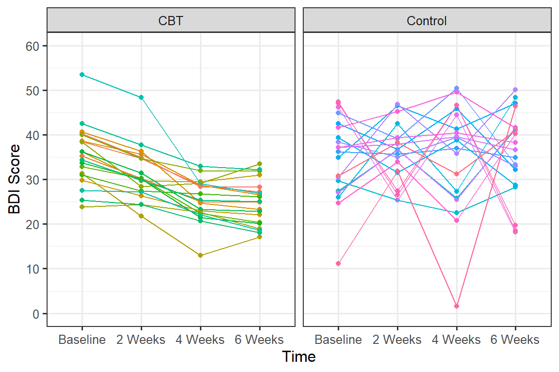
Plot of Simulation

Spaghetti Plot

Each line represents a person’s score across conditions

Means plot

Just like RM ANOVA, we will use Cousineau-Morey Corrected error bars which remove individual differences. The function will correct for the mixed design differences in the correction, just pass which variables are between below. Again, you can select between SE and CI (I plotted CI below).

#setwd("C:/Users/ademos/Dropbox/AlexFiles/teaching/UIC/Graduate/543-Fall2021/Week 11")
source('HelperFunctions.R')

MeansforGGPlot <- summarySEwithin(data=DataSim2, "BDI", 
                                  withinvars=c("Time"),
                                  betweenvars=c("Group"),
                            idvar="ID", na.rm=FALSE, conf.interval=.95)

Means.Within.CI <-ggplot(data = MeansforGGPlot, aes(x = Time, y=BDI, group=Group))+
  scale_y_continuous(breaks = seq(0,40,5))+
  geom_line(aes(colour = Group), size=2)+
  geom_ribbon(aes(ymin=BDI-ci, ymax=BDI+ci,fill = Group), alpha=.5)+
  ylab("Mean BDI Score")+xlab("Time")+
  theme(legend.position = "right")
Means.Within.CI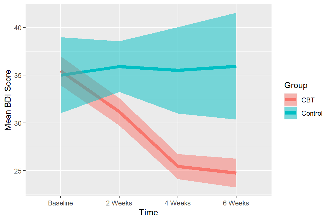

For within error bars (Corrected) you can eye-ball significance (Cumming & Finch, 2005)

95% CIs:

\(p < .05\): when proportion overlap is about .50
\(p < .01\): when proportion overlap is about 0

Notice also you can see problems with the variance

2-Way Mixed ANOVA logic

Two-way Mixed ANOVA Table With the formulas (conceptually simplified)

Source	SS	DF	MS	F
\(Between\,Subject\)	\(CSS_{row\,means}\)	\(nK-1\)	\(\frac{SS_{BS}}{df_{BS}}\)
\(Group\)	\(CnSS_{Group\,means}\)	\(K-1\)	\(\frac{SS_{G}}{df_{G}}\)	\(\frac{MS_{G}}{MS_{W_{G}}}\)
\(W_{G}\)	\(SS_{BS} - SS_{G}\)	\(K(n-1)\)	\(\frac{SS_{W_{G}}}{df_{W_{G}}}\)
\(Within\,Subject\)	\(SS_T-SS_{BS}\)	\(nK(C-1)\)	\(\frac{SS_w}{df_w}\)
\(\,RM\)	\(KnSS_{RM\,means}\)	\(C-1\)	\(\frac{SS_{RM}}{df_{RM}}\)	\(\frac{MS_{RM}}{MS_{SXRM}}\)
\(\,GXRM\)	\(nSS_{Col\,means}-SS_G-SS_{RM}\)	\((K-1)(C-1)\)	\(\frac{SS_{GXRM}}{df_{GXRM}}\)	\(\frac{MS_{GXRM}}{MS_{SXRM}}\)
\(\,Residual\,[Sub\,x\,RM]\)	\(SS_{WS}-SS_{RM}-SS_{GXRM}\)	\(K(n-1)(C-1)\)	\(\frac{SS_{SXRM}}{df_{SXRM}}\)
Total	\(SS_{scores}\)	\(N-1\)

Notes:

\(SS_{T} = SS_{BS} +SS_{WS}\)
- \(SS_{BS} = SS_{G} + SS_{W_{G}}\)
- \(SS_{WS} = SS_{RM} +SS_{GXRM} + SS_{SXRM}\)
\(df_{T} = df_{BS} +df_{WS}\)
- \(df_{BS} = df_{G} + df_{W_{G}}\)
- \(df_{WS} = df_{RM} +df_{GXRM} + df_{SXRM}\)

Explained Terms

\(SS_{G}\) = caused by group
\(SS_{RM}\) = caused by treatment
\(SS_{GXRM}\) = caused by group x treatment

Unexplained Terms

\(SS_{W_{G}}\) = Noise due to group
\(SS_{SXRM}\) = Noise due to treatment

R ANOVA Calculations

R Defaults

afex calculates the RM ANOVA for us and it will automatically correct for sphericity violations.
Error(Subject ID/RM Factor): This tells the afex that subjects vary as function RM conditions.
It reports \(\eta_g^2\) assuming a manipulated group and treatment.

library(afex)
Mixed.1<-aov_car(BDI~ Time*Group + Error(ID/Time), 
        data = DataSim2,include_aov = TRUE)
Mixed.1

## Anova Table (Type 3 tests)
## 
## Response: BDI
##       Effect          df    MSE         F  ges p.value
## 1      Group       1, 38 104.58 15.61 *** .148   <.001
## 2       Time 1.31, 49.71 108.40    4.86 * .069    .023
## 3 Group:Time 1.31, 49.71 108.40    6.10 * .085    .011
## ---
## Signif. codes:  0 '***' 0.001 '**' 0.01 '*' 0.05 '+' 0.1 ' ' 1
## 
## Sphericity correction method: GG

Assumptions

Sphericity

Same as RM ANOVA, except we should examine Mauchly’s test for Sphericity on each term (that has more than two levels)

summary(Mixed.1, return="univariate")

## 
## Univariate Type III Repeated-Measures ANOVA Assuming Sphericity
## 
##             Sum Sq num Df Error SS den Df   F value    Pr(>F)    
## (Intercept) 167941      1   3974.2     38 1605.7893 < 2.2e-16 ***
## Group         1632      1   3974.2     38   15.6057 0.0003271 ***
## Time           690      3   5388.5    114    4.8634 0.0032074 ** 
## Group:Time     865      3   5388.5    114    6.0989 0.0006928 ***
## ---
## Signif. codes:  0 '***' 0.001 '**' 0.01 '*' 0.05 '.' 0.1 ' ' 1
## 
## 
## Mauchly Tests for Sphericity
## 
##            Test statistic    p-value
## Time             0.087864 1.0173e-17
## Group:Time       0.087864 1.0173e-17
## 
## 
## Greenhouse-Geisser and Huynh-Feldt Corrections
##  for Departure from Sphericity
## 
##             GG eps Pr(>F[GG])  
## Time       0.43605    0.02332 *
## Group:Time 0.43605    0.01090 *
## ---
## Signif. codes:  0 '***' 0.001 '**' 0.01 '*' 0.05 '.' 0.1 ' ' 1
## 
##               HF eps Pr(>F[HF])
## Time       0.4453126 0.02256844
## Group:Time 0.4453126 0.01040950

Violations of Sphericity are more common in mixed designs, so be cautious

Covariance Matrix

We assume Compound Symmetry for each group:

\[ \mathbf{Cov} = \sigma^2\left[\begin{array} {rrrr} 1 & \rho & \rho & \rho \\ \rho & 1 & \rho & \rho \\ \rho & \rho & 1 & \rho \\ \rho & \rho & \rho & 1\\ \end{array}\right] \]

However, as in the case of the study that we examined today, we have two Covariance Matrices (one for each group: \(COV_1 = COV_2\)). So we must test to see if they are homogeneous. We can use Box’s M.

Box’s M

Box’s M tests to see if the covariance matrices are equal between groups (HOCV). This function in R requires we spread DV into columns based on the Within factor (we will use spread function in tidyr package: dataset %>% spread(Within factor, DV).

library(tidyr); library(dplyr); library(knitr)
#Box's M
data_wide <- DataSim2 %>% spread(Time, BDI)
kable(head(data_wide))

ID	Group	Baseline	2 Weeks	4 Weeks	6 Weeks
1	CBT	40.23859	34.86235	28.40633	28.22054
2	CBT	38.45681	34.63989	28.57209	27.19361
3	CBT	35.17345	30.23337	25.01844	24.94112
4	CBT	38.57516	35.61778	28.73243	26.55361
5	CBT	40.61921	36.26474	24.67851	23.33669
6	CBT	29.75451	26.36550	22.99378	22.10959

Now the data is wide, we will index the columns of the DV (rows 3 to 6) We will send this result to boxM function in heplots and cut it buy group. We can view the covariance matrix for each group and also view the results of the test.

library(heplots)
BoxResult<-boxM(data_wide[,3:6],data_wide$Group)
BoxResult$cov
BoxResult

## $CBT
##          Baseline  2 Weeks  4 Weeks  6 Weeks
## Baseline 44.85650 36.81309 19.53132 21.95070
## 2 Weeks  36.81309 35.33974 18.19656 15.55819
## 4 Weeks  19.53132 18.19656 21.48449 21.12618
## 6 Weeks  21.95070 15.55819 21.12618 25.09238
## 
## $Control
##           Baseline    2 Weeks    4 Weeks   6 Weeks
## Baseline  84.41210 -10.952713 105.872926 -63.09351
## 2 Weeks  -10.95271  43.060554   9.913844  51.54310
## 4 Weeks  105.87293   9.913844 146.223780 -54.50783
## 6 Weeks  -63.09351  51.543101 -54.507831  92.30349
## 
## 
##  Box's M-test for Homogeneity of Covariance Matrices
## 
## data:  data_wide[, 3:6]
## Chi-Sq (approx.) = 805.54, df = 10, p-value < 2.2e-16

Box’s M does not work well with small samples and becomes overly sensitive in large samples. We can set alpha here to be \(\alpha = .001\). If the result is significant, that means the covariance matrices are not equal which means we have a problem. This increases the rate of which we might commit a Type I error when examining the interaction: the treatment affected the covariance between trials by the group and not the just the means as we expected. So is the interaction due to mean differences or covariance differences?

HOV

Box’s M is not a great test, so its recommended you also check Levene’s test (center the data via mean) or Brown-Forsythe test (center the data via median) in the car package. Brown-Forsythe test is more robust to the violation of normality (Note: the output will still say Levene’s test when you center via median). Both these tests are sensitive to unequal sample sizes per group. We can test HOV of the groups and group*treatment. If the interaction HOV is violated it supports the conclusion of Box’s M.

library(car)
# Brown-Forsythe test on Group Only
leveneTest(BDI~ Group, data=DataSim2,center=median)

# Brown-Forsythe test on Group X Treatment Only
leveneTest(BDI~ Time*Group, data=DataSim2,center=median)

## Levene's Test for Homogeneity of Variance (center = median)
##        Df F value  Pr(>F)  
## group   1  4.4884 0.03569 *
##       158                  
## ---
## Signif. codes:  0 '***' 0.001 '**' 0.01 '*' 0.05 '.' 0.1 ' ' 1
## Levene's Test for Homogeneity of Variance (center = median)
##        Df F value   Pr(>F)   
## group   7  2.8286 0.008461 **
##       152                    
## ---
## Signif. codes:  0 '***' 0.001 '**' 0.01 '*' 0.05 '.' 0.1 ' ' 1

In the case of this study, Box’s M and Brown-Forsythe test showed HOCV and HOV problems. So we are in trouble, what can we do?

Solution?: Cohen (2008) recommends that you do not do the mixed ANOVA, meaning you will be unable to test the interaction. You can only do one-way RMs for each group and do ANOVA or independent t-tests on the groups (collapsing over RM term). Is this extremely conservative approach is it justified?

Degree of the problem?

I ran a simulation on the Type I error rates give the violations. In this simulation (n = 10,000) of 2 (between) x 4 (within) design with a sample size of 30. All the cells have mean of 0 and I let the covariance matrices for each group be random but different from each other.

Type I Levels:

Don’t Violate HOCV: Interaction term in the ANOVA (uncorrected) = .0465

Violate HOCV, but not Sphericity: Interaction term in the ANOVA (uncorrected) = .059

Violate HOCV and Sphericity: Interaction term in the ANOVA (uncorrected) = .0616

Then I followed up the significant interaction (which is a type I error!) and did a PAIRWISE comparisons (within family). Below if the number of times at least 1 follow test within each family was significant. Note: These values should be high, cause the ANOVA told you something was significant. So this would be the proportion of times, you followed up a type I error that you would get a significant type I error follow up test.

Our expected alpha for a total of 12 within tests: alpha error = 1-(1-.05)^12 = .460

Our expected alpha for a total of 4 between tests: alpha error = 1-(1-.05)^4 = .185

Approach	Correction	Don’t Violate HOCV	Violate HOCV	Violate HOCV + Sphericity
Univariate Within	None	.978	1	1
Univariate Within	Tukey	.557	.998	1
Univariate Within	Bonferroni	.492	.995	1
———————	————	———————-	————–	————-
Multivariate Within	None	.976	1	1
Multivariate Within	Tukey	.557	.998	1
Multivariate Within	Bonferroni	.480	.991	.986
———————	————	———————-	————–	————-
Univariate Between	None	.510	.844	.984
Univariate Between	Bonferroni	.211	.411	.411
———————	————	———————-	————–	————-
Multivariate Between	None	.484	.842	.836
Multivariate Between	Bonferroni	.206	.392	.413
———————	————	———————-	————–	————-
Ignore ANOVA Within	Bonferroni	.273	.338	.313
Ignore ANOVA Between	Bonferroni	.206	.364	.379
———————	————	———————-	————–	————-

Ignore ANOVA Within = paired-sample t-tests Bonferroni corrected within each group (so 6 tests per family)

Ignore ANOVA Between = Welch t-tests Bonferroni corrected within in time point (correction was .05/4)

This is the reason for Cohen suggest there are issues when following up in a non-conservative way when you violate HOCV. In the wild no one does this in practice because usually the whole point of the study. But what happens to your power?

Here is simulation (10k) where I had 88% power to detect the interaction. Below are the power numbers to detect a significant follow up from the significant interaction. Note I am showing the numbers only from the results which showed a significant interaction (so they should very high).

Approach	Correction	Violate HOCV + Sphericity
Univariate Within	None	1
Univariate Within	Tukey	1
Univariate Within	Bonferroni	1
———————	————	————-
Multivariate Within	None	1
Multivariate Within	Tukey	1
Multivariate Within	Bonferroni	1
———————	————	————-
Univariate Between	None	.960
Univariate Between	Bonferroni	.740
———————	————	————-
Multivariate Between	None	.958
Multivariate Between	Bonferroni	.730
———————	————	————-
Ignore ANOVA Within	Bonferroni	1
Ignore ANOVA Between	Bonferroni	.700
———————	————	————-

So if the interaction is NOT a type I error, your power is harmed a little by using an more conservative approach.

Recommendations

For Box’s M, set \(\alpha = .001\), double check Brown-Forsythe to be sure there is a problem, and examine Spaghetti plots when you have a small number of subjects.
- No violations:
  - It should not matter if you use the Univariate or Multivariate approach as the results will all be very close. But probably best to use a correction (Bonferroni, or Tukey if you are worried about losing too much power). You can apply the Multivariate with Bonferroni correction within Family (like SPSS)
When Box’s M & B-F are violated:
- Follow it up from the within variable ONLY and the minimum number of tests possible to test your predicted hypothesis (to protect power).
  - If you need to contrasts (using the error term of the ANOVA) do only the one you need and keep in mind you might be able to be replicated
  - If you only need pairwise tests, do NOT use the error term from the ANOVA (do paired sample t-tests and Bonferroni correct the hell out of it). You can go between, but as you see the type I error is little higher and the power is much lower (so type II problems)
  - The multivariate approach will NOT help, (but your book is correct, you should be super careful)
- DO NOT DO ANY EXPLORATORY ANALYSIS; these will be all type I error.

Basically, if you have designed your study well and had no violations, go ahead follow up the way you would follow up an RM ANOVA using emmeans, but try to follow it up only within-subject as you have higher power (and thus lower Type I risk). If you have violations and they look bad, you need to think very carefully about how to proceed.

Example of Follow up (assuming no violations)

Follow Up Interaction

Example using simple effects followed up by polynomial contrast

library(emmeans)
Time.by.Group<-emmeans(Mixed.1,~Time|Group, model="multivariate")

So changes over time in Control group which we can follow up with contrasts: polynomials, consecutive, or any custom contrast you want to test. [Note we can index 1:3 to see only the CBT results]

contrast(Time.by.Group, 'poly')

## Group = CBT:
##  contrast  estimate   SE df t.ratio p.value
##  linear     -37.885 6.98 38  -5.426  <.0001
##  quadratic    3.620 1.56 38   2.328  0.0253
##  cubic        6.479 9.00 38   0.720  0.4759
## 
## Group = Control:
##  contrast  estimate   SE df t.ratio p.value
##  linear       2.448 6.98 38   0.351  0.7278
##  quadratic   -0.478 1.56 38  -0.307  0.7603
##  cubic        2.131 9.00 38   0.237  0.8141

References

Cousineau, D., & O’Brien, F. (2014). Error bars in within-subject designs: a comment on Baguley (2012). Behavior Research Methods, 46(4), 1149-1151.

Mixed ANOVA: Two-way, Graphing & Follow ups