Power and Effect Size
Note: There is some very complex R code used to generate today’s
lecture. I have hidden it in the PDF file. If you see
echo=FALSE inside the RMD file it means that is the code
you are not expected to understand or learn. I will explain the
functions you will need to learn.
Probability is Fickle
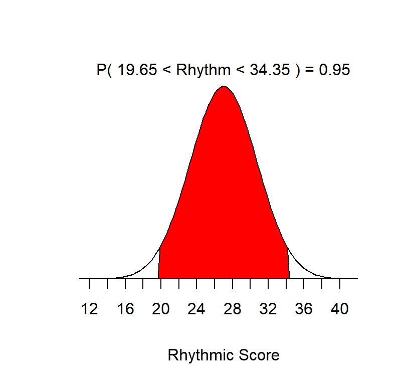
Review: The standard error can be understood as the Standard deviation of Sample Means. To understand this let’s generate a population for the Advanced Measures of Music Audiation (a test of college students tonal and rhythmic discrimination), \(\mu\) = 27, \(\sigma\) = 3.75 and view the PDF of the population. We can see below 95% of the X scores occur between about 19.65 & 34.35 on rhythmic discrimination.
Now lets draw 10 samples of \(n = 13\) people per sample. In other words, 10 data collections with 13 people where we measure their rhythmic discrimination
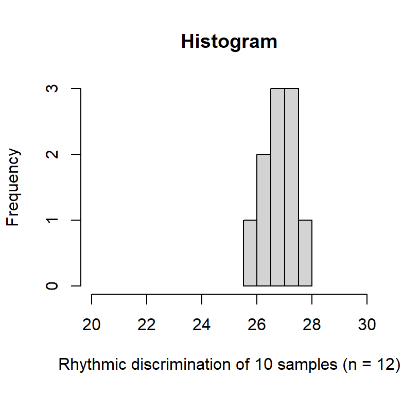
The mean of the means of the samples was 26.791, close to the mean of the popluation, \(\mu=27\). The predicted standard error based on our equation \(\sigma_M = \frac{\sigma}{\sqrt{n}} = \frac{3.75}{\sqrt{13}}\) = 1.04. In reality these 10 studies yielded SD(sample means) = 0.55. Why do different?
The problem is our original sample was too small and we probably got only people in the middle by chance. So what if we run 5000 replications of what we just did: SD(10 replications of 13 people per sample). The red line = theoretical SEM
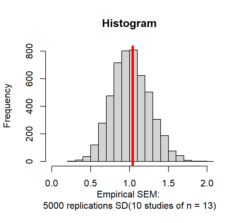
You will notice the graph is not symmetrical. In fact, 56% of the scores are below the theoretical SEM and 44% are above the theoretical SEM. Why did this happen? For the same reason, we got a low estimate before: with the small sample we are most likely getting people only from the middle of the population because they are most likely. However, sometimes by chance, you will get scores (and means) that are WAY too small or large. This the problem with Gosset introduced by moving us away from using known values of \(\sigma\) standard deviation and using the sample \(S\) as an approximation. The solution to this problem is to estimate how likely you are to get your result by chance given your specific sample size and given how big your effect is likely to be.
Signal Detection Theory
Given I must estimate my SEM from my \(S\), I need a way to see how “big” an effect might be. Cohen borrowed a useful idea at the time, signal detection theory which was created during the invention of the radio and radar. The idea was that you want to know how strong a signal needed to be for you to detect it over the noise. The noise for us is the control group and the signal the effect of your treatment.
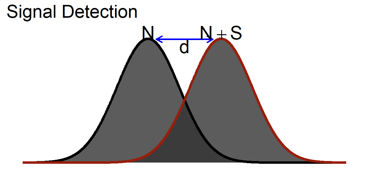
\[ d = \frac{\mu_{(Noise+Signal)}-\mu_{(Noise)}}{\sigma_{(Noise)}} \] Note this implicit assumption: \[\sigma_{(Noise)} = \sigma_{(Noise+Signal})\]
Cohen’s \(d\)
Cohen surmised that we could apply the same logic to experiments to determine how big the effect would be (in other words how easy it is to distinguish the signal from the noise).
\[ d = \frac{M_{H1}-\mu_{H0}}{S_{H1}} \]
You might notice you have seen this formula before!
\[ Z = \frac{M-\mu}{S} \]
So Cohen’s \(d\) is in standard deviation units:
| Size | \(d\) |
|---|---|
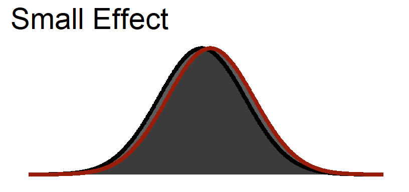
| Small | .2 |
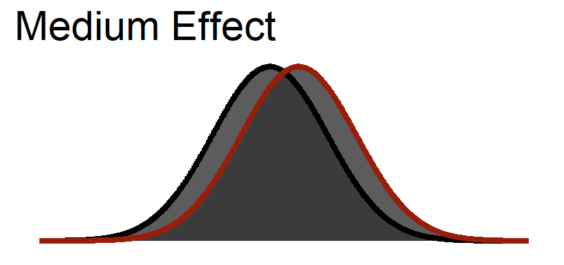
| Medium | .5 |
| Large | .8 |
Small Visualized
Medium Visualized
Large Visualized
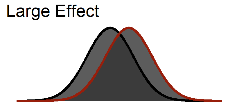
You notice that even in a large effect there is a lot of overlap between the curves.
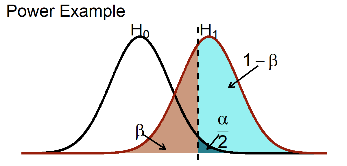
Power
Power is the likelihood that a study will detect an effect when there is an effect. Power = \(1 - \beta\), where \(\beta\) = Type II error (Cohen, 1962, 1988, 1992). Below is a visual representation of power.
Uses of Power
A priori Power: Setting a specific likelihood (power = .80) at given \(\alpha\) level (.05), knowing the true effect size. This is used to estimate the sample size needed to achieve that power (Cohen, 1962, 1988, 1992). The problem here is what is the true effect size? We used to say go find a meta-analysis to estimate it, but those effect sizes are overestimated because of publication bias (Kicinski et al., 2015). Some other rules of thumb, assume your effect is small-to-medium (d = .3 or .4).
Post-hoc Power: Estimating the power you achieved given the observed effect size you found from your study, the sample size and \(\alpha\) you set. Post-hoc power has no meaning, and the reason has to do probability being fickle (Hoenig & Heisey, 2001). In short, the problem is that your estimate of \(\sigma\) in small samples, \(S\) is going to be underestimated making your calculation of \(d\) too large. I will show you in graphs how non-trivial this issue is.
Power and Significance testing
While I have shown you power as it related to population \(\mu\) & \(\sigma\) distributions, we calculate significance testing based on ‘standard error’ units not ‘standard deviation’ units. A reminder is that this means when we say something is statistically significant it does NOT mean it is clinically significant. Example, in “Simpson and Delilah” from the Simpsons (S7:E2), Homer takes Dimoxinil, and the next morning he has a full luscious head of hair. The effect of Dimoxinil is huge! In reality, Minoxidil (the real drug) grows back very little hair (after months and months of 2x a day applications). The effect is small, but it is significant because “most” men experience hair growth beyond noise which is defined in SEM not SD.
As N increases, the standard error goes down (\(\frac{S}{\sqrt{n}}\)), meaning the width the noise decreases.
Medium Effect Size
Curves = standard deviation

Significance Test on Medium Effect size
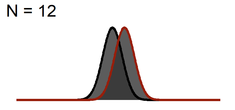
The Distance of the peaks of the curves will not change (effect size based on the graph above), but we will change the width of the curve to reflect Standard Error
Significance Test when N = 12
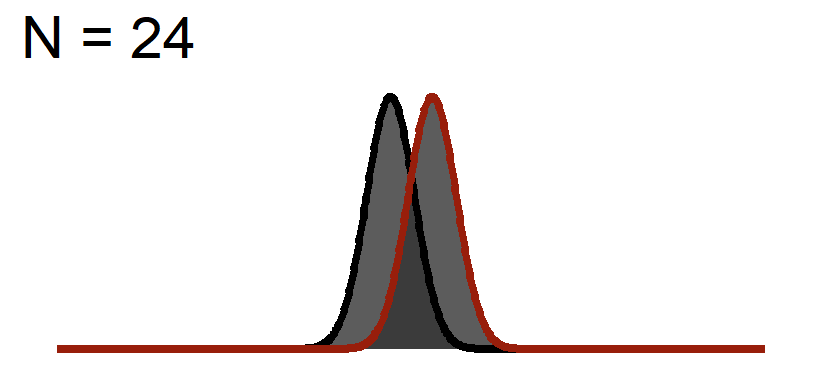
Significance Test when N = 24
Significance Test when N = 48
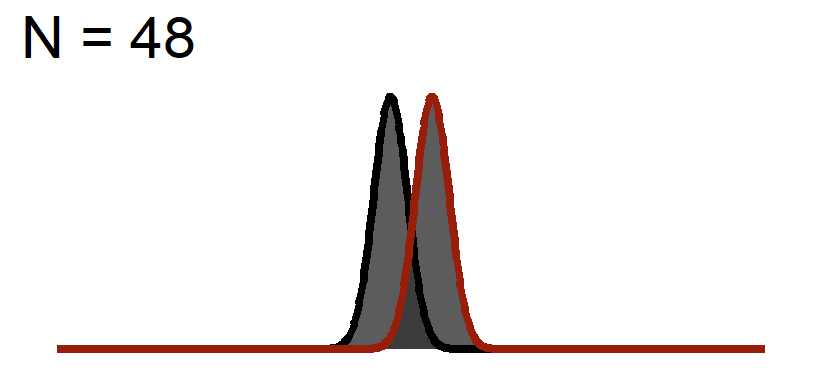
You will notice the area of \(1-\beta\) increases because as we add sample, the curve gets thinner (SEM), but the distance between them does not change! This effect size is theoretically independent of significance testing as its simply based on the mean difference / standard deviation. If you know the true standard deviation (\(\sigma\)) than this is a true statement. However, we never know the true standard deviation so we approximate it based on sample (\(S\)). So our observed estimate of effect size from experimental data is another guess based on the fickleness of probably (which is why we hope meta-analysis which averages over lots of studies is a better estimate).
Estimating A priori Power
To ensure a specific likelihood, you will find a significant effect (\(1-\beta\)) we needed to set that value. There are two values that are often chosen .8 and .95. 80% power is the value suggested by Cohen because it’s economical. 95% is called high power, and it has been favored of late (but its very expensive and you will see why). Also, you need 3 pieces of information. 1) Effect size (in Cohen’s \(d\)), 2) You \(\alpha\) level, and 3) a number of tails you want to set (usually 2-tailed).
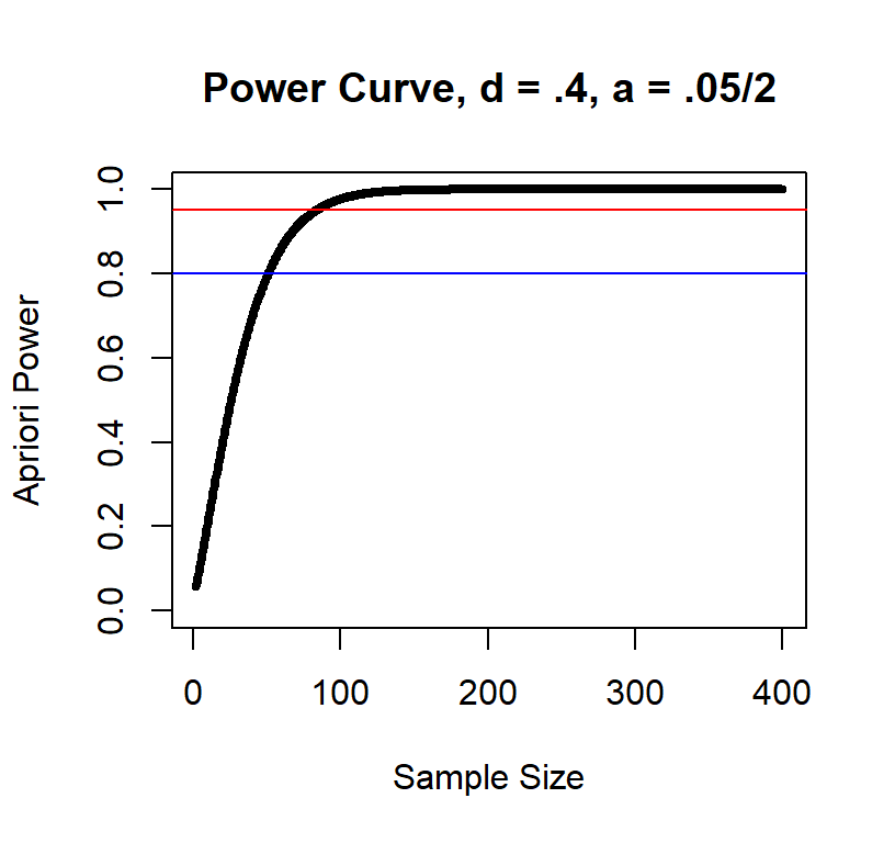
Back to our rhythmic discriminability Lets assume you create a training program to increase students rhythmic discriminability and assume the \(d\) = .4 (small-to-medium effect). We can set our \(\alpha = .05\) and number of tails (2). and let Cohen’s (1988) formulas estimate the same needed.
Power .80
pwr.t.test function in the pwr package is built into R
already (no need to install it). It is limited to what it can do, but it
can do the basic power analysis. For more complex power calculations you
will need to download gpower a free stand-alone power
software or you have to find other packages in R or build a Monte-Carlo
simulation (which I might have for you later in the semester ).
pwr.t.test works by solving what you leave as
NULL.
library(pwr)
At.Power.80<-pwr.t.test(n = NULL, d = .4, power = .80, sig.level = 0.05,
               type = c("one.sample"), alternative = c("two.sided"))
At.Power.80
##
## One-sample t test power calculation
##
## n = 51.00945
## d = 0.4
## sig.level = 0.05
## power = 0.8
## alternative = two.sidedWe round the value up 52
Power .95
At.Power.95<-pwr.t.test(n = NULL, d = .4, power = .95, sig.level = 0.05,
               type = c("one.sample"), alternative = c("two.sided"))
At.Power.95
##
## One-sample t test power calculation
##
## n = 83.16425
## d = 0.4
## sig.level = 0.05
## power = 0.95
## alternative = two.sidedWe round the value up 84
Sample size and Power
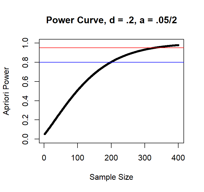
Sample size and power at a given effect size have a non-linear relationship
Power curve d = .4
Power curve d = .2
Power curve d = .8
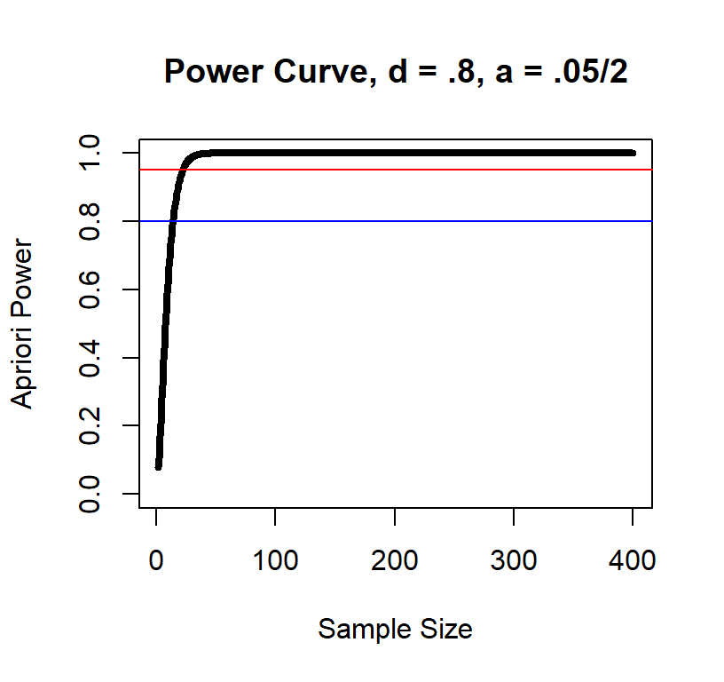
As you can see, the large the effect the fewer subjects you need.
Solve A Priori Power
You can solve A Priori power if you know your N, True d, \(\alpha\) level N = 13 d = .4 a = .05, two-tailed
library(pwr)
AP.Power.N13<-pwr.t.test(n = 13, d = .4, power = NULL, sig.level = 0.05,
               type = c("one.sample"), alternative = c("two.sided"))
AP.Power.N13
##
## One-sample t test power calculation
##
## n = 13
## d = 0.4
## sig.level = 0.05
## power = 0.2642632
## alternative = two.sidedA Priori power = 0.264
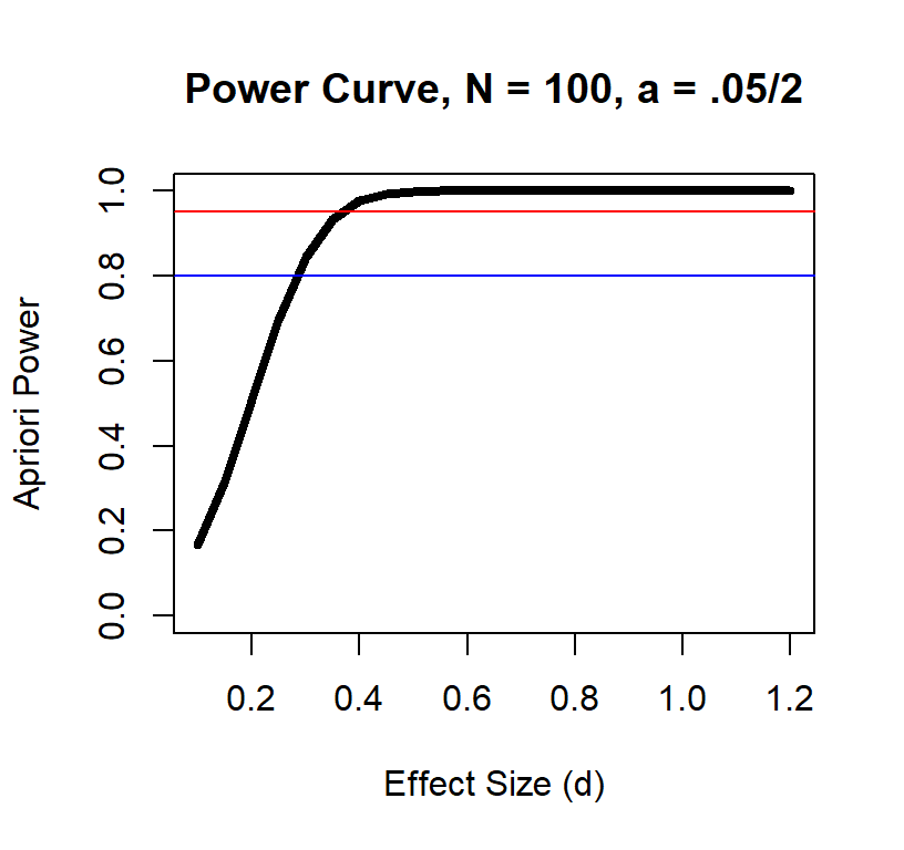
Power and Effect size
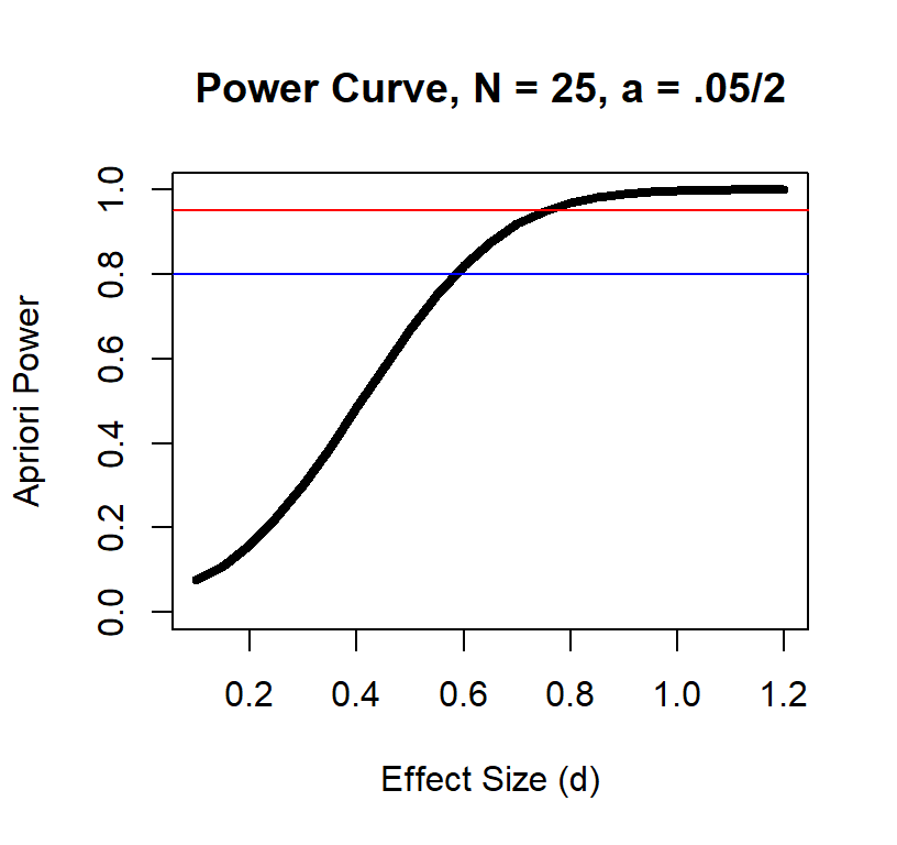
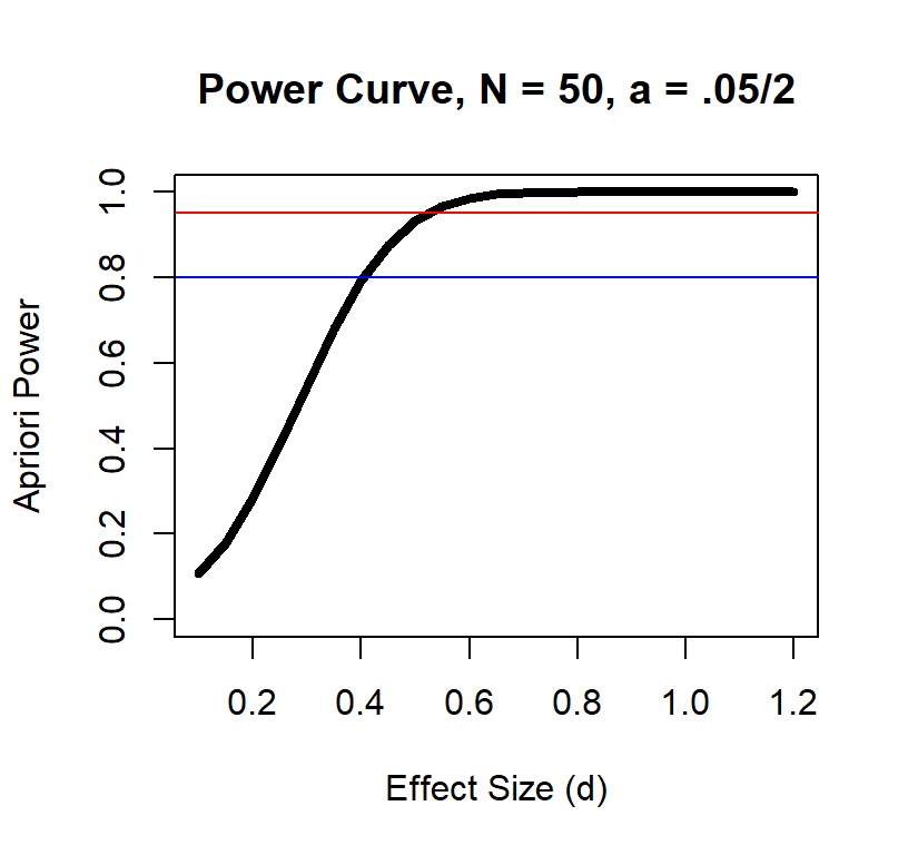
Effect size and power at a given sample size also has a non-linear relationship
Power Curve n = 25
Power Curve n = 50
Power Curve n = 100
Solve for Max Effect Size Detectable
You can solve the largest effect you can detect with your N at a specific a priori power if you know your N, Power level, \(\alpha\) level N = 13 power = .80 a = .05, two-tailed
library(pwr)
Eff.Power.N13<-pwr.t.test(n = 13, d = NULL, power = .80, sig.level = 0.05,
               type = c("one.sample"), alternative = c("two.sided"))
Eff.Power.N13
##
## One-sample t test power calculation
##
## n = 13
## d = 0.8466569
## sig.level = 0.05
## power = 0.8
## alternative = two.sidedMax Effect Size Detectable at .8 power with N = 13 is 0.847. A very high value (which is bad)
Power in independent t-tests
The function in R to similar to the functions we have been using, but now it tells you N per group. Also it assumes HOV
Let’s go back to our Mozart effect: compare IQ (spatial reasoning) of people right after they listen to Mozart’s Sonata for Two Pianos in D Major K. 448 to a control group who listened to Bach’s Brandenburg Concerto No. 6 in B flat major, BWV 1051 Concerto. If the effect is for Mozart only, we should not see it work when listening to Bach (matched on modality & tempo, and complexity of dualing voices)
Simulation: \(\mu_{Mozart} = 109\), \(\sigma_{Mozart} = 15\), \(\mu_{Bach} = 110\), \(\sigma_{Bach} = 15\), we extract a sample of \(N = 30\). Our t-test (not correcting for HOV)
# t-test
MvsB.t.test<-t.test(x= Mozart.Sample.2, y= Bach.Sample,
       alternative = c("two.sided"),
       paired = FALSE, var.equal = TRUE,
       conf.level = 0.95)
MvsB.t.test #call the results
##
## Two Sample t-test
##
## data: Mozart.Sample.2 and Bach.Sample
## t = -1.6594, df = 58, p-value = 0.1024
## alternative hypothesis: true difference in means is not equal to 0
## 95 percent confidence interval:
## -15.195895 1.420754
## sample estimates:
## mean of x mean of y
## 105.1811 112.0686Effect Size in Independent Design
We have two sources of variance group 1 and group 2. Cohen originally suggested we can simply use \(d = \frac{ M_{exp} - M_{control} }{S_{control}}\), because \(S_{control} = S_{exp}\), however later it was suggested to instead use a corrected \(d\)
\[d = \frac{M_{exp} - M_{control}}{S_{pooled}}\]
Why do you think the corrected formula is better?
Effect size package
the effsize package is useful as it can calculate \(d\) in the same way we might apply a t-test
in R.
library(effsize)

Obs.d<-cohen.d(Mozart.Sample.2, Bach.Sample, pooled=TRUE,paired=FALSE,
                   na.rm=FALSE, hedges.correction=FALSE,
                   conf.level=0.95)
Obs.d
##
## Cohen's d
##
## d estimate: -0.4284595 (small)
## 95 percent confidence interval:
## lower upper
## -0.95119710 0.09427815Note it can apply hedges correction (g)
\[g = .632\frac{M_{exp} - M_{control}}{S_{pooled}}\] Note that is am approximation to correct for small samples (note the real formula is more complex, this is just simplified version)
HedgeG<-cohen.d(Mozart.Sample.2, Bach.Sample, pooled=TRUE,paired=FALSE,
                   na.rm=FALSE, hedges.correction=TRUE,
                   conf.level=0.95)
HedgeG
##
## Hedges's g
##
## g estimate: -0.4228951 (small)
## 95 percent confidence interval:
## lower upper
## -0.9386945 0.0929044Estiamte sample size at Power .80
Lets say our d = 0.423
ID.At.Power.80<-pwr.t.test(n = NULL, d = abs(HedgeG$estimate), power = .80, sig.level = 0.05,
               type = c("two.sample"), alternative = c("two.sided"))
ID.At.Power.80
##
## Two-sample t test power calculation
##
## n = 88.74578
## d = 0.4228951
## sig.level = 0.05
## power = 0.8
## alternative = two.sided
##
## NOTE: n is number in *each* groupWe round the value up 89 and that is the number we need PER GROUP assuming this effect size estimated from our failed experiment.
Estimate sample size at Power .95
ID.At.Power.95<-pwr.t.test(n = NULL, d = abs(HedgeG$estimate), power = .95, sig.level = 0.05,
               type = c("two.sample"), alternative = c("two.sided"))
ID.At.Power.95
##
## Two-sample t test power calculation
##
## n = 146.2894
## d = 0.4228951
## sig.level = 0.05
## power = 0.95
## alternative = two.sided
##
## NOTE: n is number in *each* groupWe round the value up 147 and that is the number we need PER GROUP assuming this effect size estimated from our failed experiment.
Problem with Observed d
Running a single pilot with a small sample to estimate the effect size was a standard practice. However, it can result in problems. We got a small effect size by chance. What if we re-run our study (N = 30) 5000 times?
In theory my true d = \(110 - 109 / 15\) = .067. Basically a zero effect. When people look at \(d\) they tend to take the absolute value (we will do the same)
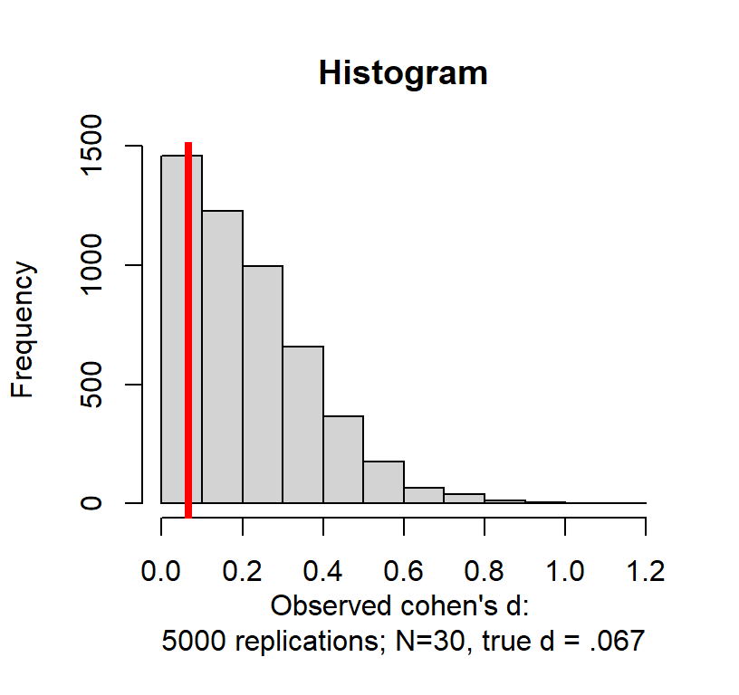
So in fact our estimated d from that one experiment (observed d = 0.428 had a 10.6% chance of occurring! Worse yet, there was a 46.32% chance of getting a value above a small effect \(d = .2\)
References
Cohen, J. (1962). The statistical power of abnormal-social psychological research: A review. The Journal of Abnormal and Social Psychology, 65, 145-153.
Cohen, J. (1988). Statistical power analysis for the behavioral sciences (2nd edition). Hillsdale, NJ: Lawrence Erlbaum Associates.
Cohen, J. (1992). A power primer. Psychological Bulletin, 112, 155-159.
Hoenig, J. M., & Heisey, D. M. (2001). The abuse of power: the pervasive fallacy of power calculations for data analysis. The American Statistician, 55, 19-24.
Kicinski, M., Springate, D. A., & Kontopantelis, E. (2015). Publication bias in meta-analyses from the Cochrane Database of Systematic Reviews. Statistics in medicine, 34(20), 2781-2793.
Note: Power graphs adapted from: http://rpsychologist.com/creating-a-typical-textbook-illustration-of-statistical-power-using-either-ggplot-or-base-graphics