Multiple Comparisons (Bonferroni vs FDR)
Review: Philosophy I (Familywise) Correction for Error Rate
Dominant Philosophy in Experimental Psychology
| Declared | Null is True (no difference) | Null is False (difference) | Total |
|---|---|---|---|
| Sig | Type 1 (V) | True Positives (S) | R |
| Non-Sig | True Negative (U) | Type II (T) | M-R |
| Total | Mo | M-Mo | M |
Familywise error = V / Mo = Probability of getting at least one test wrong
Simulation of FWER
Let’s imagine that 25% of the brain region are different from each other at a set effect size. We will run a Monte-Carlo Simulation: 50,000 t-tests, \(N=10\) per group, \(\alpha_{pc}=.05\), which will yield Power = .50. Our goal is to find those 25 regions and we will assume each test is independent and we sample with replacement. Further, we will know which regions were actually different (We know the “truth”).
Results Table of FWER Simulation
| Declared | Null is True (no difference) | Null is False (difference) | Total |
|---|---|---|---|
| Sig | 1829 | 6281 | 8110 |
| Non-Sig | 35671 | 6219 | 41890 |
| Total | 37500 | 12500 | 50000 |
FWER = V / Mo = 0.049
Type II = T/M-Mo = 0.498, which is correct since power = .50
If you ran 10K studies 16.22% of them would have been declared significant (R/M), but in reality 25% of the studies had a true effect.
Here is another way to view it: Of the tests we declared significant a large percentage of them of were not real (V / R = 22.55%).
Bonferroni Correction
\[\alpha_{pc} = \frac{\alpha_{EW}}{j} = \frac{.05}{50,000} = 1X10^{-6} \]
We will keep everything else the same from the last simulation.
Results Table of Bonferroni Simulation
| Declared | Null is True (no difference) | Null is False (difference) | Total |
|---|---|---|---|
| Sig | 0 | 3 | 3 |
| Non-Sig | 37500 | 12497 | 49997 |
| Total | 37500 | 12500 | 50000 |
FWER = V / Mo = 0
Type II = T/M-Mo = 1. So we missed everything (power is basically 0)
So we made no mistakes, but we found nothing. NIH never gives you another penny.
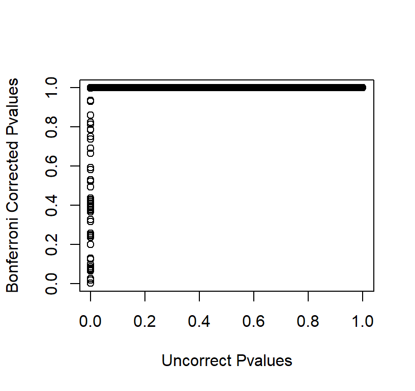
Plot of Bonferroni Corrected Pvalues
Increase Power, Rinse and Repeat
Given our original d = 0.926, we would recalculate the sample size we would need per group (62) given our new alpha \(\alpha_{pc} = 5X10^{-6}\). That is a 520% increase in sample size!
Let’s try to increase our sample size to 62 per group and try again
Results Table of Higher Powered Bonferroni Simulation (Power = .5)
| Declared | Null is True (no difference) | Null is False (difference) | Total |
|---|---|---|---|
| Sig | 0 | 6339 | 6339 |
| Non-Sig | 37500 | 6161 | 43661 |
| Total | 37500 | 12500 | 50000 |
FWER = V / Mo = 0
Type II = T/M-Mo = 0.493. So we fixed our power problem and made no FWER! BUT:
650 Per scan * N = 10 * 2 groups = 13,000 dollars
650 Per scan * N = 62 * 2 groups = 80,600 dollars
And yet we still miss 50% of the results because we are powered at .50. If we go to power .95, as we don’t want to miss 50% of the results.
N = 106
650 Per scan * N = 106 * 2 groups = 137,800 dollars
Results Table of Super Powered Bonferroni Simulation (Power = .95)
| Declared | Null is True (no difference) | Null is False (difference) | Total |
|---|---|---|---|
| Sig | 0 | 11906 | 11906 |
| Non-Sig | 37500 | 594 | 38094 |
| Total | 37500 | 12500 | 50000 |
FWER = V / Mo = 0
Type II = T/M-Mo = 0.048.
All of the low low price of 137,800 dollars for 1 study!
Philosophy II False Rate of Discovery
FWER is appropriate when you want NO false positives
Dominant Philosophy in Neuroscience, genomics, etc. Any field where they are not as worried about false positives but interested in making discoveries.
| Declared | Null is True (no difference) | Null is False (difference) | Total |
|---|---|---|---|
| Sig | Type 1 (V) | True Positives (S) | R |
| Non-Sig | True Negative (U) | Type II (T) | M-R |
| Total | Mo | M-Mo | M |
FDR error = V / R
Benjamini and Hochberg procedure
- Sort all p-values from all tests you did (smallest to largest)
- Assign ranks to the p-values (lowest=1, etc.).
- Calculate each individual p-value’s Benjamini-Hochberg critical value, using the formula (rank/total number of tests)*q, where: q = the false discovery rate (a percentage, chosen by you or via algorithm which is beyond our scope)
- Compare your original p-values to the B-H critical value; find the largest pvalue that is smaller than the critical value.
For example 5 t-tests only:
| Test | Pvalue | Rank | BH Critical Value (Rank/m)*q [.1] | Significant? |
|---|---|---|---|---|
| Test 5 | .001 | 1 | 0.02 | Yes |
| Test 1 | .030 | 2 | 0.04 | Yes |
| Test 3 | .045 | 3 | 0.06 | Yes |
| Test 2 | .056 | 4 | 0.08 | Yes |
| Test 4 | .230 | 4 | 0.1 | No |
FDR simulation
Repeat our original simulation but correct the pvalues using FDR correction. Note we will set FDR level to be about .05 to compare to Bonferroni, but people could change their alpha to be higher (.1 or .25 as in the Dead Salmon Paper).
Results Table of FDR Simulation
| Declared | Null is True (no difference) | Null is False (difference) | Total |
|---|---|---|---|
| Sig | 21 | 633 | 654 |
| Non-Sig | 37479 | 11867 | 49346 |
| Total | 37500 | 12500 | 50000 |
We can compare this to our Bonferroni Correction Table.
FDR = V / R = 0.0321
Type II = T/M-Mo = 0.949
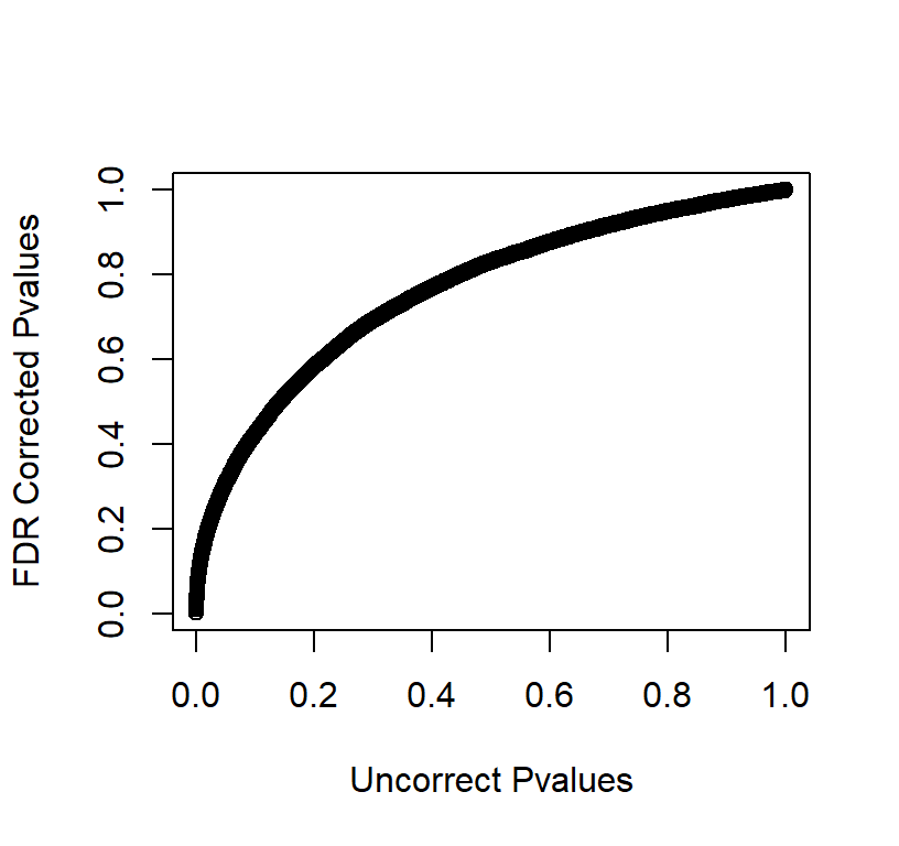
Plot of FDR Corrected Pvalues
Results Table of FDR Simulation (alpha=.10)
| Declared | Null is True (no difference) | Null is False (difference) | Total |
|---|---|---|---|
| Sig | 152 | 1958 | 2110 |
| Non-Sig | 37348 | 10542 | 47890 |
| Total | 37500 | 12500 | 50000 |
We can compare this to our Bonferroni Correction Table.
FDR = V / R = 0.072
Type II = T/M-Mo = 0.843
Notes
- FDR q values are controlled via an algorithm in R, and we will not go into the details.
- FDR (BH procedure) is only one of methods, there are others, but we will not go into them.
- FDR correction is often applied to correction matrices because it’s
more logical as you are doing exploratory work. Simply pass your pvalues
into this function:
Correct.Pvalues<-p.adjust(Pvector, method = 'fdr'). You can decide on what to call significant (alpha .05 or .10 depending on how exploratory you want to be). - To avoid these issues, FMRI hypothesis can be constrained to be not “whole brain” or voxel by voxel comparisons.