Design Example for Last Class

Kardas & O’Brien (2018) recently reported that with the proliferation of YouTube videos, people seem to think they can learn by seeing rather than doing. They “hypothesized that the more people merely watch others, the more they believe they can perform the skill themselves.” They compared extensively watching the “tablecloth trick” with extensively reading or thinking about it. Participants assessed their own abilities to perform the “tablecloth trick.” Participants were asked to rate from 1 (I feel there’s no chance at all I’d succeed on this attempt) to 7 (I feel I’d definitely succeed without a doubt on this attempt). The study was a 3 (type of exposure: watch, read, think) ? 2 (amount of exposure: low, high) between-subjects design. They collected an N = 1,003 with small effect sizes (\(n^2 <.06\)), but to make this analysis doable by hand I will cut the same to 5 people per cell and inflate the effect size (but keep the pattern the same as their experiment 1).

Low Exposure Group Watching Reading Thinking Row Means
\(\,\) 1 3 3
\(\,\) 3 2 3
\(\,\) 3 3 2
\(\,\) 4 1 3
\(\,\) 2 4 1
———————— ——— ———- ———- ———-
Cell Means 2.6 2.6 2.4 2.53
Cell SS 5.2 5.2 3.2
High Exposure Group Watching Reading Thinking Row Means
\(\,\) 6 5 3
\(\,\) 4 3 2
\(\,\) 7 2 1
\(\,\) 5 3 4
\(\,\) 5 2 4
———————— ——— ———- ———- ———-
Cell Means 5.4 3.0 2.8 3.73
Cell SS 5.2 6.0 6.8
Column Means 4.0 2.8 2.6 G = 3.13

ANOVA Result

library(afex)

Anova.Results<-aov_car(Perceived.Ability~Level*Type + Error(ID), 
                  data=Example.Data)
Anova.Results
## Anova Table (Type 3 tests)
## 
## Response: Perceived.Ability
##       Effect    df  MSE       F  ges p.value
## 1      Level 1, 24 1.32 8.20 ** .255    .009
## 2       Type 2, 24 1.32  4.35 * .266    .024
## 3 Level:Type 2, 24 1.32  3.65 * .233    .041
## ---
## Signif. codes:  0 '***' 0.001 '**' 0.01 '*' 0.05 '+' 0.1 ' ' 1

Follow Up Logic

Just like the one-way ANOVA, the two-way ANOVA tells us which factors are different, but not which levels. The best approach to follow is the Hybrid approach: Do the Confirmatory approach (planned comparisons). Test anything exploratory as conservatively as you can (unplanned comparisons). You need to carefully distinguish what you are doing to your reader.

The challenge of the two-way ANOVA is unpacking a significant interaction. All interaction must be unpacked, meaning they must be explained (which cells have driven the effect). This is not always easy the interaction may not always come out as predicted.

Basic Rules

  • Do not follow up F-tests that were not significant
  • Use error term from ANOVA to do contrasts or protected-t
  • Planned: no multiple comparison correction necessary if under 3 tests, but can be applied if you want to be conservative or have multiple planned tests
  • Unplanned: apply multiple comparison correction
  • Interactions: DO as FEW TESTS as possible to explain the interaction (don’t follow it up both ways)

Hypothesis from Example data

Kardas and O’Brien (2018) hypothesized that spending more time watching YouTube videos would cause someone to think the can do the tablecloth trick. Therefore, from their hypothesis, we would predict that the degree of exposure would impact only the watched condition: the high exposure group to should have a higher mean on watched over the low exposure group, but no differences between low and high exposure on reading or thinking about the trick. In sum, they are predicting only 2 cells differ (Low vs High @ Watched). Note: Non-significant mean no significant difference (cannot reject null). It does not mean the groups are the same. Be careful about talking about non-significant results.

Main Effects vs Interaction

If the interaction is telling a conflicting story with the main effects, you may either not want to follow up the main effects or carefully explain them. You will notice in Kardas & O’Brien (2018) they did not follow up the main effects, only the interaction.

Planned Comparisons of Interaction

Simple Effects with 2-Levels

They want to test the simple effects (one factor at the level of another factor) of Level of Exposure at each Type of Exposure. AKA: Low vs. High @ Watching, Low vs. High @ Reading, Low vs. High @ Thinking.

Just like when we followed up the one-way ANOVA, we will use the df and error term from omnibus ANOVA (\(df_W\) & \(MS_W\)). To do this, we will use emmeans package. Note: These can be reported as F-tests (as basically, we are doing one-way ANOVAs) or as t-values. Dont get confused as this is the sample calculation as before when followed up one-way ANOVA, but we now following up an interaction.

As F-tests (one-way ANOVAs)

Here is the old fashioned way (By hand method). Run a one-way ANOVA at each level of one of the variables (such as Type) and than re-calculate the F and p-value using the error term of the omnibus model). We would need to recalculate the effect size as well.

\[F = \frac{MS_{Level_{oneway}}}{MS_{W_{omnibus}}}\] We need to subset the data to only have Type==Watching

Example.Data.WatchingOnly<-subset(Example.Data, Type=="Watching")

One_way.Watching<-aov_car(Perceived.Ability~Level + Error(ID), 
                  data=Example.Data.WatchingOnly)
One_way.Watching
## Anova Table (Type 3 tests)
## 
## Response: Perceived.Ability
##   Effect   df  MSE        F  ges p.value
## 1  Level 1, 8 1.30 15.08 ** .653    .005
## ---
## Signif. codes:  0 '***' 0.001 '**' 0.01 '*' 0.05 '+' 0.1 ' ' 1

Problem is the error term is incorrect, so we need to extract the \(SS_{levels}\), convert it to \(MS_{levels} = \frac{SS_L}{df_L}\) and redivide by the omnibus ANOVA error terms (\(MS_W\)).

SS_L.Watch<-One_way.Watching$Anova$`Sum Sq`[2]
DF_L.Watch<-One_way.Watching$Anova$Df[2]
MS_L.Watch<- SS_L.Watch/DF_L.Watch

MS_W<-Anova.Results$anova_table$MSE[1]

F_Watch <- MS_L.Watch/ MS_W
P_Watch <- pf(F_Watch, 1, 24, lower.tail = FALSE)

Next we would have to recalculate the effect size by hand.

\[\eta_{p_{Levels}}^2 = \frac{SS_L}{SS_L + SS_W}\]

SSw.watch<-Anova.Results$Anova$`Sum Sq`[5]

Eta_p_Watch <- SS_L.Watch/(SS_L.Watch+SSw.watch)

Simple effect for watching, F(1,24) = 14.886, p < 8^{-4}, \(\eta^2_p\) = 0.38

You would report this process 2 more times for each level of TYPE. The fast way to do it is via emmeans!

Fit Model via emmeans

First, we must cut the ANOVA we calculated the way we want to test the results:

library(emmeans)
library(dplyr)
Simple.Effects.By.Type<-emmeans(Anova.Results, ~Level|Type)
Simple.Effects.By.Type
## Type = Watching:
##  Level emmean    SE df lower.CL upper.CL
##  Low      2.6 0.513 24     1.54     3.66
##  High     5.4 0.513 24     4.34     6.46
## 
## Type = Reading:
##  Level emmean    SE df lower.CL upper.CL
##  Low      2.6 0.513 24     1.54     3.66
##  High     3.0 0.513 24     1.94     4.06
## 
## Type = Thinking:
##  Level emmean    SE df lower.CL upper.CL
##  Low      2.4 0.513 24     1.34     3.46
##  High     2.8 0.513 24     1.74     3.86
## 
## Confidence level used: 0.95

In this case the F-tests = squared(t-values). All we have to do is call the joint_test function. This will run 3 one-way ANOVAs using the DF and error terms from the two-way ANOVA automatically.

As F

One_way.By.Type<-joint_tests(Anova.Results, by = "Type")
One_way.By.Type
## Type = Watching:
##  model term df1 df2 F.ratio p.value
##  Level        1  24  14.886  0.0008
## 
## Type = Reading:
##  model term df1 df2 F.ratio p.value
##  Level        1  24   0.304  0.5866
## 
## Type = Thinking:
##  model term df1 df2 F.ratio p.value
##  Level        1  24   0.304  0.5866

Notice: Our “by hand values” match.

As t-values

In this case, we have 2 level within each Exposure, thus we can report it instead as t-tests in this case (the answers will exactly the same). You see above; we have 3 subsets of the results. Now we can calculate the F-values, and we can use the pairs function. This will run 3 LSD tests (protected t-tests) using the DF and error terms from the two-way ANOVA automatically.

pairs(Simple.Effects.By.Type,adjust='none') %>% summary(infer = TRUE)
## Type = Watching:
##  contrast   estimate    SE df lower.CL upper.CL t.ratio p.value
##  Low - High     -2.8 0.726 24     -4.3     -1.3  -3.858  0.0008
## 
## Type = Reading:
##  contrast   estimate    SE df lower.CL upper.CL t.ratio p.value
##  Low - High     -0.4 0.726 24     -1.9      1.1  -0.551  0.5866
## 
## Type = Thinking:
##  contrast   estimate    SE df lower.CL upper.CL t.ratio p.value
##  Low - High     -0.4 0.726 24     -1.9      1.1  -0.551  0.5866
## 
## Confidence level used: 0.95

We can use the same code before to calculate Cohen’s d to match our t-value. If we want \(\eta_{p}^2\) would need to calculate it instead by hand (I cannot find a way to do it via the package yet).

Effect size

SD.pooled = sqrt(Anova.Results$anova_table$MSE)[1]
eff_size(Simple.Effects.By.Type, sigma = SD.pooled, edf = 24, method='pairwise')
## Type = Watching:
##  contrast   effect.size    SE df lower.CL upper.CL
##  Low - High      -2.440 0.724 24    -3.93   -0.946
## 
## Type = Reading:
##  contrast   effect.size    SE df lower.CL upper.CL
##  Low - High      -0.349 0.634 24    -1.66    0.961
## 
## Type = Thinking:
##  contrast   effect.size    SE df lower.CL upper.CL
##  Low - High      -0.349 0.634 24    -1.66    0.961
## 
## sigma used for effect sizes: 1.147 
## Confidence level used: 0.95

Note: These are seen 3 families of 1 test. So even if you try to apply FWER you cannot.

As t-values (contrast approach)

You can also call a contrast code and get the same exact results. Note: this will be useful as we add more levels.

Set1 <- list(
  H1 = c(-1,1))

contrast(Simple.Effects.By.Type,Set1,adjust='none')
## Type = Watching:
##  contrast estimate    SE df t.ratio p.value
##  H1            2.8 0.726 24   3.858  0.0008
## 
## Type = Reading:
##  contrast estimate    SE df t.ratio p.value
##  H1            0.4 0.726 24   0.551  0.5866
## 
## Type = Thinking:
##  contrast estimate    SE df t.ratio p.value
##  H1            0.4 0.726 24   0.551  0.5866

Which to report?

F or t values? When you use the words “simple effects” or “contrasts” people are primed to see F-values (and people generally don’t ask for FWER corrections). When you pairwise approach, they think you are doing unprotected t-tests and want to see FWER.

Following up the interaction the other way

First and foremost, ONLY UNPACK THE INTERACTION WITH ONE FAMILY OF SIMPLE EFFECTS. Do not think you now also have to test it the other way: Watching vs. Reading vs. Thinking @ Low, Watching vs. Reading vs. Thinking @ High. You will notice in their paper they did not do this as they did not hypothesize these type of follow-ups. Also, they already Unpacked their ANOVA. They know what caused the interaction. Any additional tests are merely a waste of time and will inflate FWER. Now, might you have a hypothesis that was very complex and required you to follow it both ways? Yes, you would limit which simple effects you would examine to those you need to see to understand the effects.

Simple Effects with 3-Levels

They did not hypothesize following up the other way, but we will do it anyway as an example of how to do it. The problem we have is that we have three level: Watching vs Reading vs Thinking @ Low, Watching vs Reading vs Thinking @ High. In the old school approach, we first have to run an F-test (one-way ANOVA) at each level of Level of Exposure and run pairwise or contrasts to follow up if the One-way was significant.

Fit Model via emmeans

First, we must cut the ANOVA we calculated the way we want to test the results:

One_way.Level<-joint_tests(Anova.Results, by = "Level")
One_way.Level
## Level = Low:
##  model term df1 df2 F.ratio p.value
##  Type         2  24   0.051  0.9507
## 
## Level = High:
##  model term df1 df2 F.ratio p.value
##  Type         2  24   7.949  0.0022

Because there are three level you cannot ever run these as t-tests. Also, the package will not easily give you effect sizes. Luckly with between-subject ANOVAs its easy to convert your F values over to effect sizes. Note: This will NOT work the same was a more complex designs (mixed or repeated measures).

You can convert the F values into \(\eta_{p}^2\). [Formula from your textbook]

\[\eta_{p}^2 = \frac{df_bF}{df_bF+df_w}\] Note: Since we have 2 F values, we can get R to give us 2 effect sizes!

Fs = One_way.Level$F.ratio
df_b = One_way.Level$df1
df_w =One_way.Level$df2

eta_p_exposure<- (Fs * df_b)/(Fs * df_b + df_w)
eta_p_exposure
## [1] 0.004232014 0.398466089

Simple effect for Low, F(2,24) = 0.051, p < 0.9507, \(\eta^2_p\) = 0.0042

Simple effect for High, F(2,24) = 7.949, **p* < 0.0022, \(\eta^2_p\) = 0.3985

So we have a simple effect of High exposure. We would need to follow this effect up to see which is different. The degree of correction you use will depend on if its planned or unplanned comparison.

Follow up of Significant Simple Effect

The code will run these are 2 families of 3 tests. You need to ignore the results of the low exposure group.

Specific Contrasts

Pairwise approach, specific to only significant simple effect you want to follow up (and apply some correction)

Simple.Effects.at.Level<-emmeans(Anova.Results, ~Type+Level)
Simple.Effects.at.Level

Set2 <- list(
  High.EvsR = c(0,0,0,-1,1,0),
  High.WvsT = c(0,0,0,-1,0,1),
  High.RvsT = c(0,0,0,0,-1,1))

contrast(Simple.Effects.at.Level,Set2,adjust='MVT')
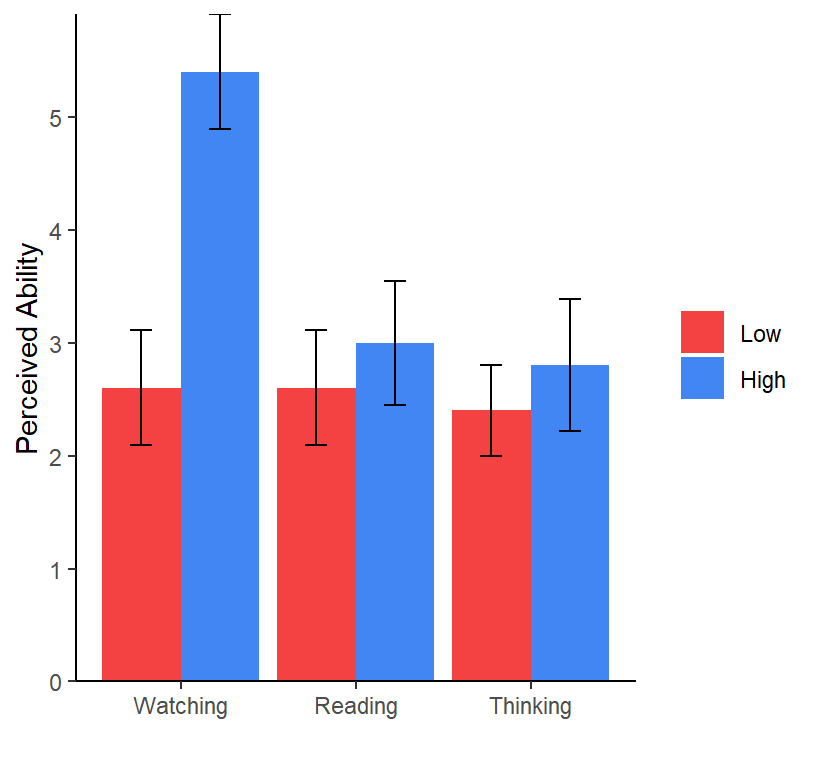
##  Type     Level emmean    SE df lower.CL upper.CL
##  Watching Low      2.6 0.513 24     1.54     3.66
##  Reading  Low      2.6 0.513 24     1.54     3.66
##  Thinking Low      2.4 0.513 24     1.34     3.46
##  Watching High     5.4 0.513 24     4.34     6.46
##  Reading  High     3.0 0.513 24     1.94     4.06
##  Thinking High     2.8 0.513 24     1.74     3.86
## 
## Confidence level used: 0.95 
##  contrast  estimate    SE df t.ratio p.value
##  High.EvsR     -2.4 0.726 24  -3.307  0.0081
##  High.WvsT     -2.6 0.726 24  -3.583  0.0042
##  High.RvsT     -0.2 0.726 24  -0.276  0.9591
## 
## P value adjustment: mvt method for 3 tests

Simplier, but less control

It will correct for 3 tests per family (almost same at MVT). Note its corrected per family. So you would need to ignore the low group.

Simple.Effects.by.Level<-emmeans(Anova.Results, ~Type|Level)
pairs(Simple.Effects.by.Level,adjust='tukey')
## Level = Low:
##  contrast            estimate    SE df t.ratio p.value
##  Watching - Reading       0.0 0.726 24   0.000  1.0000
##  Watching - Thinking      0.2 0.726 24   0.276  0.9591
##  Reading - Thinking       0.2 0.726 24   0.276  0.9591
## 
## Level = High:
##  contrast            estimate    SE df t.ratio p.value
##  Watching - Reading       2.4 0.726 24   3.307  0.0080
##  Watching - Thinking      2.6 0.726 24   3.583  0.0041
##  Reading - Thinking       0.2 0.726 24   0.276  0.9591
## 
## P value adjustment: tukey method for comparing a family of 3 estimates

“Complex” Linear Contrast

Here you can merge and compare groups as before. You can apply corrections if you lots of tests, but they will be within the family: Bonferroni, Sidak, mvt, or FDR.

Simple.Effects.at.Level<-emmeans(Anova.Results, ~Type+Level)

Set3 <- list(
  WvsRT = c(0,0,0,1,-.5,-.5))

contrast(Simple.Effects.at.Level,Set3,adjust='none')
##  contrast estimate    SE df t.ratio p.value
##  WvsRT         2.5 0.628 24   3.978  0.0006

“Consecutive” Contrast

If the data were ordinal, you could test them in some kind of logical order. You can apply corrections if you lots of tests, but they will be within the family: Bonferroni, Sidak, mvt, or FDR.

Consec.Set <- list(
  WvsR = c(-1,1,0),
  RvsT = c(0,-1,1))

contrast(Simple.Effects.by.Level,Consec.Set,adjust='none')
# Also 
# contrast(Simple.Effects.By.Level,'consec',adjust='none')
## Level = Low:
##  contrast estimate    SE df t.ratio p.value
##  WvsR          0.0 0.726 24   0.000  1.0000
##  RvsT         -0.2 0.726 24  -0.276  0.7852
## 
## Level = High:
##  contrast estimate    SE df t.ratio p.value
##  WvsR         -2.4 0.726 24  -3.307  0.0030
##  RvsT         -0.2 0.726 24  -0.276  0.7852

“Polynomial” Contrast

If the data were ordinal, you could test to see if they have a linear slope or curvilinear slope. You can apply corrections if you lots of tests, but they will be within the family: Bonferroni, Sidak, mvt, or FDR.

Poly.Set <- list(
  Linear = c(-1,0,1),
  Quad = c(-.5,1,-.5))

contrast(Simple.Effects.by.Level,Poly.Set,adjust='none')
# Also 
# contrast(Simple.Effects.By.Level,'poly',adjust='none')
## Level = Low:
##  contrast estimate    SE df t.ratio p.value
##  Linear       -0.2 0.726 24  -0.276  0.7852
##  Quad          0.1 0.628 24   0.159  0.8749
## 
## Level = High:
##  contrast estimate    SE df t.ratio p.value
##  Linear       -2.6 0.726 24  -3.583  0.0015
##  Quad         -1.1 0.628 24  -1.750  0.0929

Main-effect Follow up

Remember, we would not follow this one up because of the hypothesis we are testing, but you may want to follow up the main effects in other cases. If this is planned, go with less stringent correction. If its unplanned use a more conservative correction.

Code wise it the same as we did for one-way ANOVA, here we can only follow up the Type of Exposure. Again we will use the df and error term from the two-way interaction.

Main.Effects.Type<-emmeans(Anova.Results, ~Type)
Main.Effects.Type
##  Type     emmean    SE df lower.CL upper.CL
##  Watching    4.0 0.363 24     3.25     4.75
##  Reading     2.8 0.363 24     2.05     3.55
##  Thinking    2.6 0.363 24     1.85     3.35
## 
## Results are averaged over the levels of: Level 
## Confidence level used: 0.95

You can run the pairwise or any of the contrast approaches I showed you for interactions.

pairs(Main.Effects.Type,adjust='tukey')
##  contrast            estimate    SE df t.ratio p.value
##  Watching - Reading       1.2 0.513 24   2.338  0.0695
##  Watching - Thinking      1.4 0.513 24   2.728  0.0304
##  Reading - Thinking       0.2 0.513 24   0.390  0.9200
## 
## Results are averaged over the levels of: Level 
## P value adjustment: tukey method for comparing a family of 3 estimates

Unplanned Comparisons

This is all the same code as above, but you should use conservative corrections. There are also ways to force R to recognize there are more tests within the family but we will not cover that today.

References

Kardas, M., & O’Brien, E. (2018). Easier Seen Than Done: Merely Watching Others Perform Can Foster an Illusion of Skill Acquisition. Psychological science, 29(4), 521-536.