Main-Effects
\(H_0\): All groups have equal means
\(H_1\): At least 1 group is different from the other
Kardas & O’Brien (2018) recently reported that with the proliferation of YouTube videos, people seem to think they can learn by seeing rather than doing. They “hypothesized that the more people merely watch others, the more they believe they can perform the skill themselves.” They compared extensively watching the “tablecloth trick with extensively reading or thinking about it. Participants assessed their own abilities to perform the”tablecloth trick.” Participants were asked to rate from 1 (I feel there’s no chance at all I’d succeed on this attempt) to 7 (I feel I’d definitely succeed without a doubt on this attempt). The study was a 3 (type of exposure: watch, read, think) X 2 (amount of exposure: low, high) between-subjects design. They collected an N = 1,003 with small effect sizes (\(n^2 <.06\)), but to make this analysis doable by hand I will cut the same to 5 people per cell and inflate the effect size (but keep the pattern the same as their experiment 1).
| Low Exposure Group | Watching | Reading | Thinking | Row Means |
|---|---|---|---|---|
| \(\,\) | 1 | 3 | 3 | |
| \(\,\) | 3 | 2 | 3 | |
| \(\,\) | 3 | 3 | 2 | |
| \(\,\) | 4 | 1 | 3 | |
| \(\,\) | 2 | 4 | 1 | |
| ———————— | ——— | ———- | ———- | ———- |
| Cell Means | 2.6 | 2.6 | 2.4 | 2.53 |
| Cell SS | 5.2 | 5.2 | 3.2 |
| High Exposure Group | Watching | Reading | Thinking | Row Means |
|---|---|---|---|---|
| \(\,\) | 6 | 5 | 3 | |
| \(\,\) | 4 | 3 | 2 | |
| \(\,\) | 7 | 2 | 1 | |
| \(\,\) | 5 | 3 | 4 | |
| \(\,\) | 5 | 2 | 4 | |
| ———————— | ——— | ———- | ———- | ———- |
| Cell Means | 5.4 | 3.0 | 2.8 | 3.73 |
| Cell SS | 5.2 | 6.0 | 6.8 | |
| Column Means | 4.0 | 2.8 | 2.6 | G = 3.13 |
We now have two factors, and we will test the main effects and interaction.
\(H_0\): All groups have equal means
\(H_1\): At least 1 group is different from the other
\(H_0\): There is no interaction between factors A and B. All the mean differences between treatment conditions are explained by the main effects.
\(H_1\): There is an interaction between factors A and B. The mean differences between treatment conditions are not what would be predicted from the overall main effects of the two factors.
One-way ANOVA has Only one factor to test: \(SS_T = SS_{W}+SS_{B}\)
Two-way ANOVA has multiple factors to test: \(SS_T = SS_{W}+ (SS_{FactorA}+SS_{FactorB}+SS_{AxB})\)
Note that in the two-way ANOVA: \(SS_B = (SS_{FactorA}+SS_{FactorB}+SS_{AxB})\)
Omnibus F (same as one-way)
\[F= \frac{MS_{B}}{MS_{W}}\]
This will still tell is if one cell is different from another, but we also have to calculate F-tests on Factors A, B, and the AxB
\[F= \frac{MS_{FactorA}}{MS_{W}}\] \[F= \frac{MS_{FactorB}}{MS_{W}}\] \[F= \frac{MS_{AXB}}{MS_{W}}\]
With the formulas (formal equations)
| Source | SS | DF | MS | F |
|---|---|---|---|---|
| Between | \(n\displaystyle\sum_{i=1}^{k}(M_i-G)^2\) | \(K-1\) | \(\frac{SS_B}{df_B}\) | \(\frac{MS_B}{MS_W}\) |
| Within | \(\displaystyle \sum_{i=1}^{K}\sum_{j=1}^{n}(X_{i_{j}}-M_i)^2\) | \(N-K\) | \(\frac{SS_W}{df_W}\) | |
| Total | \(\displaystyle\sum_{j=1}^{N}(X_j-G)^2\) | \(N-1\) |
With the formulas (conceptually simplified)
| Source | SS | DF | MS | F |
|---|---|---|---|---|
| Between | \(nSS_{treatment}\) | \(K-1\) | \(\frac{SS_B}{df_B}\) | \(\frac{MS_B}{MS_W}\) |
| Within | \(\displaystyle \sum SS_{within}\) | \(N-K\) | \(\frac{SS_W}{df_W}\) | |
| Total | \(SS_{scores}\) | \(N-1\) |
Note: \(SS_B + SS_W = SS_T\) & \(df_B + df_W = df_T\)
| Source | SS | DF | MS | F |
|---|---|---|---|---|
| Between | \(SS_B\) | \(df_B\) | \(MS_B\) | F |
| \(Factor\,A_{Row}\) | \(SS_r\) | \(df_r\) | \(MS_r\) | F |
| \(Factor\,B_{Col}\) | \(SS_c\) | \(df_c\) | \(MS_c\) | F |
| \(Factor\,AxB\) | \(SS_{rxc}\) | \(df_{rxc}\) | \(MS_{rxc}\) | F |
| Within | \(SS_W\) | \(df_W\) | \(MS_W\) | |
| Total | \(SS_T\) | \(df_T\) |
With the formulas (formal equations)
| Source | SS | DF | MS | F |
|---|---|---|---|---|
| Between | \(\tiny n\displaystyle\biggl(\sum_{w=1}^{r}(M_r-G)^2+\sum_{u=1}^{c}(M_c-G)^2\biggr)\) | \(rc-1\) | \(\frac{SS_B}{df_B}\) | \(\frac{MS_B}{MS_W}\) |
| \(\,A_{(Rows)}\) | \(\tiny n_r\displaystyle\sum_{w=1}^{r}(M_w-G)^2\) | \(r-1\) | \(\frac{SS_r}{df_r}\) | \(\frac{MS_r}{MS_W}\) |
| \(\,B_{(Col)}\) | \(\tiny n_c\displaystyle\sum_{u=1}^{c}(M_u-G)^2\) | \(c-1\) | \(\frac{SS_c}{df_c}\) | \(\frac{MS_c}{MS_W}\) |
| \(\,AxB\) | \(\tiny SS_{B}-(SS_r-SS_c)\) | \((r-1)(c-1)\) | \(\frac{SS_{rxc}}{df_{rxc}}\) | \(\frac{MS_{rxc}}{MS_W}\) |
| Within | \(\tiny \displaystyle \sum_{w=1}^{r}\sum_{j=1}^{n}(X_{w_{j}}-M_w)^2+\displaystyle \sum_{u=1}^{c}\sum_{j=1}^{n}(X_{u_{j}}-M_u)^2\) | \(nrc-rc\) | \(\frac{SS_w}{df_w}\) | |
| Total | \(\tiny \displaystyle\sum_{j=1}^{N}(X_j-G)^2\) | \(nrc-1\) |
With the formulas (conceptually simplified)
| Source | SS | DF | MS | F |
|---|---|---|---|---|
| Between | \(nSS_{all\,cell\,means}\) | \(rc-1\) | \(\frac{SS_B}{df_B}\) | \(\frac{MS_B}{MS_W}\) |
| \(\,A_{(Rows)}\) | \(n_rSS_{row\,means}\) | \(r-1\) | \(\frac{SS_r}{df_r}\) | \(\frac{MS_r}{MS_W}\) |
| \(\,B_{(Cols)}\) | \(n_cSS_{col\,means}\) | \(c-1\) | \(\frac{SS_c}{df_c}\) | \(\frac{MS_c}{MS_W}\) |
| \(\,AxB\) | \(\tiny SS_{B}-(SS_r-SS_c)\) | \((r-1)(c-1)\) | \(\frac{SS_{rxc}}{df_{rxc}}\) | \(\frac{MS_{rxc}}{MS_W}\) |
| Within | \(\displaystyle \sum SS_{within}\) | \(nrc-rc\) | \(\frac{SS_w}{df_w}\) | |
| Total | \(SS_{scores}\) | \(nrc-1\) |
Note for SS: \(SS_B + SS_W = SS_T\) & \(SS_B = SS_r + SS_c+ SS_{rxc}\)
Note for DF: \(df_B + df_W = df_T\) & \(df_B = df_r + df_c+ df_{rxc}\)
Just like one-way ANOVA, we will use eta-squared = proportion of variance the treatment accounts for. Remember \(SS_B\) is the variation caused by treatment, and \(SS_T\) is the variation of Treatment + Noise.
\[\eta_B^2 = \frac{SS_B}{SS_B+SS_W} = \frac{SS_B}{SS_T}\]
\[\eta_r^2 = \frac{SS_r}{SS_T}\]
\[\eta_c^2 = \frac{SS_c}{SS_T}\]
\[\eta_{rxc}^2 = \frac{SS_{rxc}}{SS_T}\]
Eta-squared the = proportion of the total (variance) pie this effect is accounting for. The nice thing is that eta-squared adds can be used to add up to 100%! However, the values calculated thus depend upon the number of other effects and the magnitude of those other effects.
People often prefer to report Partial Eta-Squared, \(\eta_p^2\) = ratio: effect / error variance that is attributable to the effect. This “controls” for the other effects and reports what the effect is relative to the noise (not total). This is “ratio” where eta-squared was a “proportion”. Thus you cannot sum them up to 100%.
\[\eta_{p_{r}}^2 = \frac{SS_r}{SS_T-(SS_c-SS_{rxc})}\]
\[\eta_{p_{c}}^2 = \frac{SS_c}{SS_T-(SS_r-SS_{rxc})}\]
\[\eta_{p_{rxc}}^2 = \frac{SS_{rxc}}{SS_T-(SS_r-SS_c)}\]
This Partial Eta-Squared formula for two-way ANOVA is equal to the more modern generalized-eta squared \(\eta^2_g\) that R automatically generates (in the case that between subject treatment conditions were manipulated). When they are not-manipulated (like gender) that formulas change a bit which we will talk about next week along with \(\omega^2_g\) for bias correction.
I build our data frame by hand in the long format.
n=5; r=2; c=3;
Example.Data<-data.frame(ID=seq(1:(n*r*c)),
          Level=c(rep("Low",(n*c)),rep("High",(n*c))),
          Type=rep(c(rep("Watching",n),rep("Reading",n),rep("Thinking",n)),2),
          Percieved.Ability = c(1,3,3,4,2,3,2,3,1,4,3,3,2,3,1,
                                6,4,7,5,5,5,3,2,3,2,3,2,1,4,4))

# Also, I want to re-set the order using the `factor` command and set the order I want.
Example.Data$Level<-factor(Example.Data$Level,
                              levels = c("Low","High"),
                              labels = c("Low","High"))

Example.Data$Type<-factor(Example.Data$Type,
                              levels = c("Watching","Reading","Thinking"),
labels = c("Watching","Reading","Thinking"))library(dplyr)
Means.Table<-Example.Data %>%
group_by(Level,Type) %>%
summarise(N=n(),
Means=mean(Percieved.Ability),
SS=sum((Percieved.Ability-Means)^2),
SD=sd(Percieved.Ability),
SEM=SD/N^.5)
knitr::kable(Means.Table, digits = 2)
# Note remember knitr::kable makes it pretty, but you can just call `Means.Table`| Level | Type | N | Means | SS | SD | SEM |
|---|---|---|---|---|---|---|
| Low | Watching | 5 | 2.6 | 5.2 | 1.14 | 0.51 |
| Low | Reading | 5 | 2.6 | 5.2 | 1.14 | 0.51 |
| Low | Thinking | 5 | 2.4 | 3.2 | 0.89 | 0.40 |
| High | Watching | 5 | 5.4 | 5.2 | 1.14 | 0.51 |
| High | Reading | 5 | 3.0 | 6.0 | 1.22 | 0.55 |
| High | Thinking | 5 | 2.8 | 6.8 | 1.30 | 0.58 |
Normally we plot bar graphs with 1 SEM unit. I used the object I
created Means.Table that has the means. A We will apply
some fancy code to make our plot more APA!
library(ggplot2)

Plot.1<-ggplot(Means.Table, aes(x = Type, y = Means, group=Level))+
  geom_col(aes(group=Level, fill=Level), position=position_dodge(width=0.9))+
  scale_y_continuous(expand = c(0, 0))+ # Forces plot to start at zero
  geom_errorbar(aes(ymax = Means + SEM, ymin= Means - SEM),
                position=position_dodge(width=0.9), width=0.25)+
  scale_fill_manual(values=c("#f44141","#4286f4"))+
  xlab('')+
  ylab('Percieved Ability')+
  theme_bw()+
  theme(panel.grid.major=element_blank(),
        panel.grid.minor=element_blank(),
        panel.border=element_blank(),
        axis.line=element_line(),
        legend.title=element_blank())
Plot.1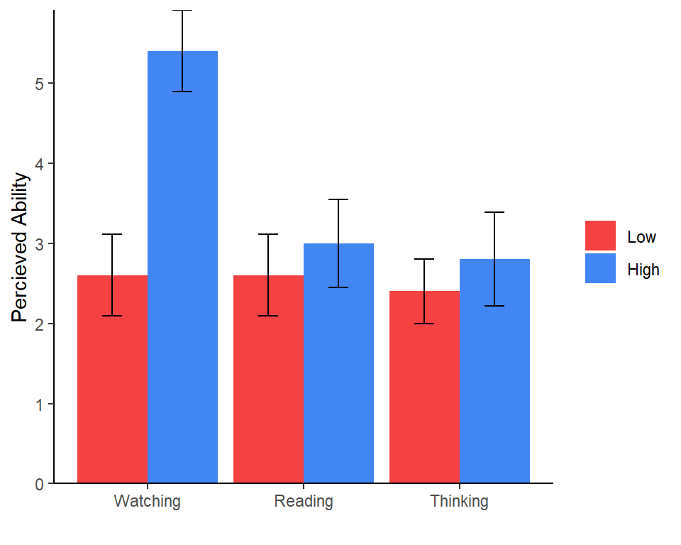
Which effects do you predict will be significant?
Again, we will use the afex package developed to allow
people to do SPSS-like ANOVA in R (Type III).
library(afex)

ANOVA.JA.Table<-aov_car(Percieved.Ability~Level*Type + Error(ID),
                  data=Example.Data, return='Anova')
ANOVA.JA.Table| Sum Sq | Df | F value | Pr(>F) | |
|---|---|---|---|---|
| (Intercept) | 294.53333 | 1 | 223.696202 | 0.0000000 |
| Level | 10.80000 | 1 | 8.202532 | 0.0085526 |
| Type | 11.46667 | 2 | 4.354430 | 0.0243529 |
| Level:Type | 9.60000 | 2 | 3.645570 | 0.0414456 |
| Residuals | 31.60000 | 24 | NA | NA |
nice)library(afex)
Nice.JA.Table<-aov_car(Percieved.Ability~Level*Type + Error(ID),
data=Example.Data)
Nice.JA.Table## Anova Table (Type 3 tests)
##
## Response: Percieved.Ability
## Effect df MSE F ges p.value
## 1 Level 1, 24 1.32 8.20 ** .255 .009
## 2 Type 2, 24 1.32 4.35 * .266 .024
## 3 Level:Type 2, 24 1.32 3.65 * .233 .041
## ---
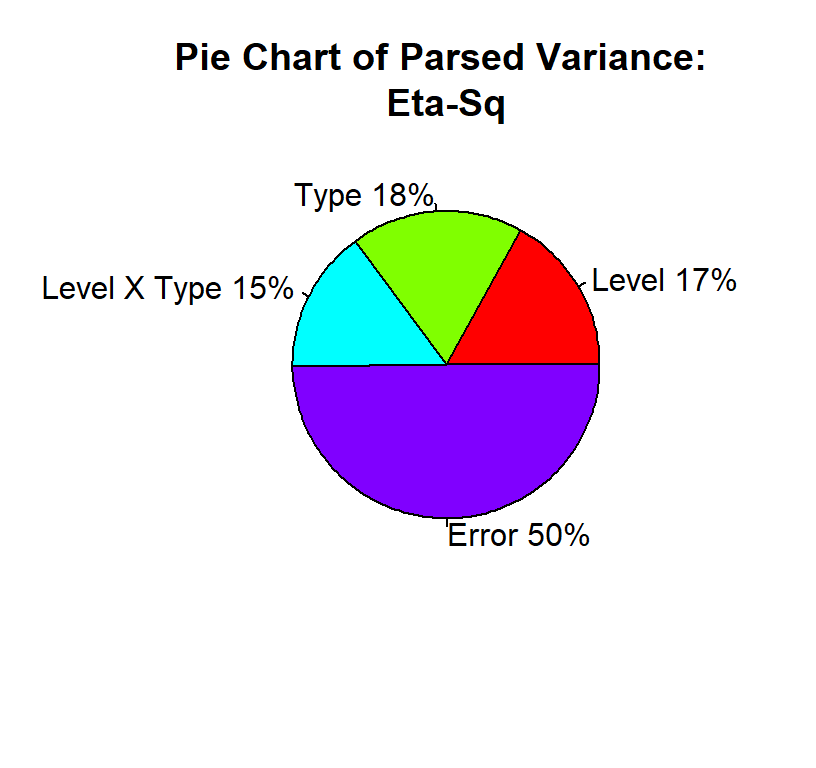
## Signif. codes: 0 '***' 0.001 '**' 0.01 '*' 0.05 '+' 0.1 ' ' 1\(\eta^2\) is a useful method for understanding how your ANOVA “parsed” your variance, but not always as useful to report in papers
Here we see that Type, Level, and Type X Level are “Explained Variance”. In total, you explained about 50% of the variance. The error term is “Unexplained Variance” (the residual). It is important you do not confuse \(\eta^2\) (the chart below) with \(\eta_p^2\).
We assume HOV and normality. We can test for HOV using Levene’s test formula, which is like the Brown-Forsythe test we used for one-way ANOVA, but we can apply it multiple factors.
Using the car package, we can test our violations. Just
like Brown-Forsythe, you do NOT want this test to be significant.
library(car)
leveneTest(Percieved.Ability ~ Level*Type, data = Example.Data) | Df | F value | Pr(>F) | |
|---|---|---|---|
| group | 5 | 0.1170732 | 0.9873727 |
| 24 | NA | NA |
Often we examine QQ plots of the DV. If the data points are very different from the line, it suggests violations of normality.
qqnorm(Example.Data$Percieved.Ability)
qqline(Example.Data$Percieved.Ability)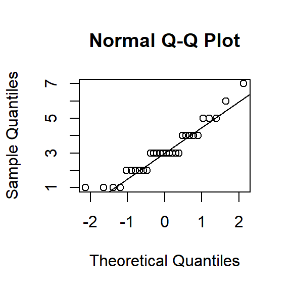
Shapiro-Wilk test is a way of testing normality statistically, but this is the test is very sensitive especially in small samples. You do NOT want this test to be significant. In our case it is, but our sample is really small.
shapiro.test(Example.Data$Percieved.Ability)##
## Shapiro-Wilk normality test
##
## data: Example.Data$Percieved.Ability
## W = 0.92911, p-value = 0.04649Kardas, M., & O’Brien, E. (2018). Easier Seen Than Done: Merely Watching Others Perform Can Foster an Illusion of Skill Acquisition. Psychological science, 29(4), 521-536.